Download PDF
Download page Task 1. Incorporating regional skew into a Bulletin 17C analysis.
Task 1. Incorporating regional skew into a Bulletin 17C analysis
Overview
This tutorial provides an example application of incorporating regional skew (using weighted skew) in a Bulletin 17C flow-frequency analysis. Regional skew, when available, is used to improve the probability distribution estimates for a site.
HEC-SSP version 2.3.1 was used to create this example. You will need HEC-SSP version 2.3.1, or newer, to open the project files.
Download a copy of the initial HEC-SSP project here: RegionalSkew_Start.zip
Introduction
The site used for this example is the St. Francis River at Patterson, Missouri. This stream gage has a drainage area of 956 square miles. The period of record used in this analysis is 99 years (WY 1921–2019). A Bulletin 17C analysis using just the at-site skew, referred to as the station skew, will be compared with an analysis using weighted skew of the station skew and a regional skew estimate.

Open the RegionalSkew.ssp project in HEC-SSP.
The plot below shows the annual maximum series of instantaneous (peak) flow for the St. Francis River gage. You can view this time series by right-clicking on the ST FRANCIS RIVER-PATTERSON,MO-FLOW-ANNUAL PEAK data in the project and selecting Plot.

Create a Bulletin 17C Analysis using Station Skew
- Create a new Bulletin 17 analysis with the name "St Francis_Station Skew". Select the ST FRANCIS RIVER flow data set from the drop down.
- Make sure the 17C EMA method and the Use Station Skew generalized skew methods are selected. Do not make any other changes to the General tab.
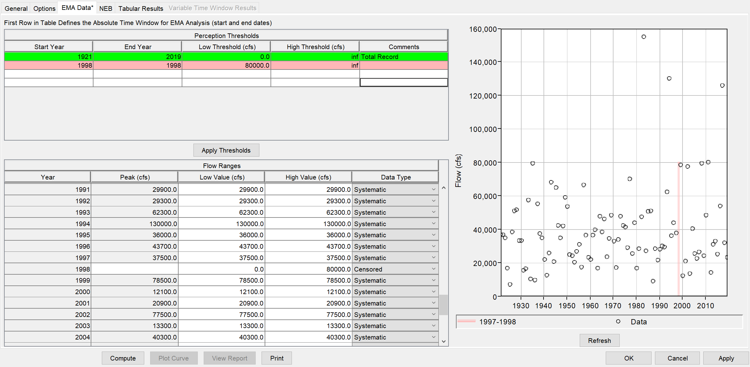
- Select the EMA Data tab. Check for any periods of missing data. There is one missing data point in 1998. From past flood reports, it is known that the 1998 flood event did not exceed 80,000 cfs. Fill in the Perception Thresholds table to include the year 1998 with a Low Threshold of 80,000 cfs. Select Apply Thresholds. The table and plot should resemble the figure below.
- Select Compute to run the B17C analysis.
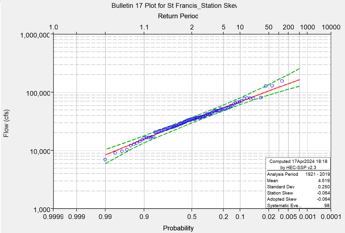
- View results using Plot Curve and in the Tabular Results tab.
The number of systematic events is 98 years, with an ERL of 98.7 years (due to the missing event in 1998). The threshold set for the 1998 event provides less information than one year worth of systematic data.
The station skew is -0.064.
Look Up Regional Skew
Regional skew, also referred to as generalized skew, is estimated by pooling data from many gages in a homogeneous population to gain the effect of a larger sample size. The regionalized skew estimate is combined with an at-site skew estimate through a weighting procedure outlined in Bulletin 17C.
The U.S. Geological Survey has performed numerous regional skew studies for various locations in the U.S., often on a state-by-state basis. For the St. Francis River, which is located in southeastern Missouri, a USGS regional skew analysis was performed for the state of Missouri in 2014. A regional skew coefficient was estimated using Bayesian weighted least-squares/generalized least-squares regression analyses using 108 stream gages with at least 30 years of record.
Link to the USGS report: https://pubs.usgs.gov/sir/2014/5165/
PDF of the USGS report: USGS_2014_Rural_Missouri_Regional_Study.pdf
Citation: Southard, R.E., and Veilleux, A.G., 2014, Methods for estimating annual exceedance-probability discharges and largest recorded floods for unregulated streams in rural Missouri: U.S. Geological Survey Scientific Investigations Report 2014–5165, 39 p., http://dx.doi.org/10.3133/sir20145165.
Navigate to the USGS report and locate the regional skew estimate for Missouri, as well as the mean square error (MSE) of the estimate. Regional skew can be found on page 6 and the Appendix (page 30).
The regional skew value is -0.30, and the mean square error (MSE) is 0.14.
This analysis investigated 35 basin characteristics as possible independent variables in the regression analysis. However, no variables were identified as statistically significant. Therefore a constant model was used for the entire study area. Most regional skew studies in the U.S. use a constant skew model.
Create a Bulletin 17C Analysis using Weighted Skew
- Create a copy of the "St Francis_Station Skew" and name it "St Francis_Weighted Skew". To create a copy, right-click on the analysis name and select Save As.
- Under the General tab, select the Use Weighted Skew radio button. Input the regional skew of -0.30 and the MSE of 0.14 that were determined from the USGS regional skew study.
- Verify there is no missing data in the EMA Data tab, then hit Compute.
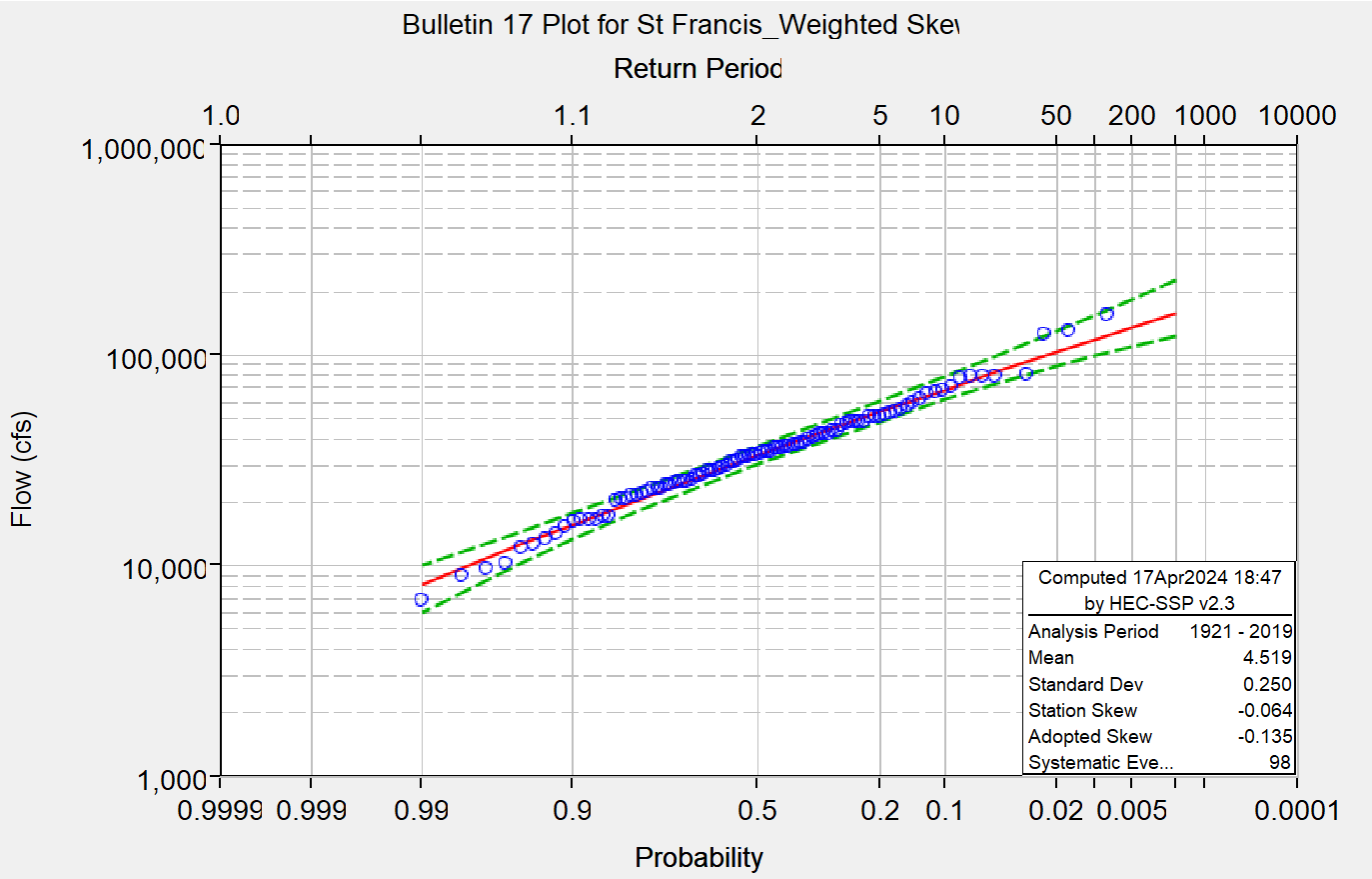
- View results using Plot Curve and in the Tabular Results tab.
The number of systematic events is 98 years, with an ERL of 110.5 years. The regional skew added approximately 12 years of information to the analysis.
The weighted skew is -0.135.
Compare Results
To view the plotted results together, highlight both analyses and select Results | Graph.
In the plot below, the analysis using station skew is displayed in green, and the analysis using weighted skew is displayed in purple.
The inclusion of regional skew shifted the adopted skew estimate from -0.064 to -0.135. Note this shifted the computed curve slightly further (lower) from the three largest events. The assumption is that the sample is not large enough to accurately represent the population, and that the inclusion of regional skew will improve the accuracy of the estimate even if the curve does not appear to fit the systematic data as well.
Additionally, note the change in the magnitude of the confidence bounds. The inclusion of regional skew increased the effective record length which resulted in slightly smaller confidence bounds (i.e., lower uncertainty).

Download the Task 1 final files here: RegionalSkew_Task1.zip