Download PDF
Download page Task 4. Bulletin 17C | Systematic Record + Historical Information + Paleoflood Information.
Task 4. Bulletin 17C | Systematic Record + Historical Information + Paleoflood Information
Return to Task 3. Bulletin 17C | Systematic Record + Historical Information.
Disclaimer: The information presented within this workshop is for instructional purposes only and does not represent any actual studies undertaken by the United States Army Corps of Engineers. All dates presented are relative to the completion date of the paleoflood analysis which was completed in 2018.
Background Information
A paleoflood analysis was completed for the Big Sandy River near Bruceton, TN. This study was undertaken in an effort to provide geologic and hydrologic information related to large historic and pre-historic discharges. The work was completed through a collaborative effort among geologic, geomorphic, hydraulic, and hydrologic disciplines using state-of-science methods. The analysis yielded evidence of a high-stage flood deposit and evidence of features that have not been eroded or deposited upon during the past several hundred years.
The analytical approach involved field identification of geologic and geomorphic evidence of past large floods (i.e., paleostage indicators, PSI) or evidence of surface stability and a lack of inundation (i.e., non-exceedance bounds, NEB). The elevations of two river terraces (i.e., called the “Qt1” and “Qt2” terraces, from oldest to youngest) were delineated using high-resolution topographic data and compared with discharge estimates from HEC-RAS two-dimensional hydraulic modeling. A schematic representation of NEB and PSI within a cross section is shown in the following figure.
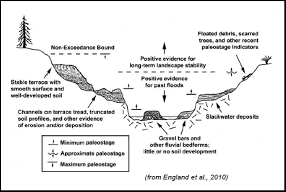
Geomorphic and stratigraphic evidence show that the Qt1 terrace has not been eroded or deposited upon since its formation approximately 600 – 800 years ago. The age estimate of the Qt1 terrace deposit is based on relative soil-profile development, radiocarbon analyses of charcoal fragments, and Optically Stimulated Luminescence analyses of river sand deposits. The estimated paleodischarge capable of inundating the Qt1 terrace is within a range of 75,000 to 250,000 cfs. The Qt1 terrace can be interpreted as a NEB.
Additionally, deposits associated with the Qt2 terrace, which is inset into and younger than the Qt1 terrace, may represent a subsequent, intermediate flood. The Qt2 terrace is interpreted to have been formed approximately 170 years ago (with a range of about 150 – 250 years ago), from the same suite of dating techniques. The estimated paleodischarge needed to inundate this surface and result in deposition of silty sand is within a range of 25,000 to 70,000 cfs). The Qt2 terrace can be interpreted as a PSI (i.e. discrete event not within the historic record).
Using the skills that you have acquired, you must now interpret the results of this paleoflood analysis and include them to estimate the 1-, 0.5,-, 0.2-, 0.1-, 0.01-, and 0.001-percent chance exceedance peak flow rates. This information will be used to size and design critical infrastructure related to an ongoing Feasibility Study.
Create a New Bulletin 17 Analysis
Project Files
Continue using the project files from Task 3, or alternatively download them here:
- Open the HEC-SSP project.
- Right click on the existing “BigSandyRiver_Historical_B17C” analysis.
- Click Save As…
- Name the new analysis “BigSandyRiver_Paleo_B17C” and add an adequate description.
Ensure you have selected the newly created analysis before making changes.
- Ensure that the “BigSandyRiver” data set is selected.
- Select “17C EMA” within the Method for Computing Statistics and Confidence Limits
- Utilize the default selections of Use Station Skew, Multiple Grubbs-Beck low outlier test, and Hirsch/Stedinger plotting position.
Add Additional Ordinates
- Move to the Options
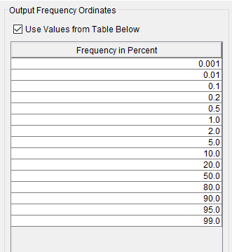
- Check the box to Use Values from Table Below within the Output Frequency Ordinates panel.
- Right click and select Insert Row(s)…
- Elect to insert 3 rows.
- Enter 0.1, 0.01, 0.001 (in ascending order) within the new, blank rows.
Utilize the Right Click | Sort Ordinates function to sort in ascending order.
- The Output Frequency Ordinates panel should should resemble the following figure.
Input EMA Data
- Move to the EMA Data
- Ensure that the historic event information for 1897, 1919, and 1926 events are included within the Flow Ranges
- Ensure that the Data Type for all of these events is set to Historical.
- Ensure that the Perception Thresholds table contains a row with “1897”, “1929”, “18000”, and “inf” for the Start Year, End Year, Low Threshold, and High Threshold entered, respectively.
- Ensure that the Perception Thresholds table contains a row with “1988”, “2002”, “18000”, and “inf” for the Start Year, End Year, Low Threshold, and High Threshold entered, respectively.
The first row of the Perception Thresholds table controls the time window of the entire analysis. Since we’d like to include paleoflood information possibly dating back to the year ~1200, the first row of the Perception Thresholds table needs to be modified.
- Change the first row in the Perception Thresholds table so that the analysis spans your interpreted date range of the NEB. ***It is possible that your interpretation of the age of the NEB will differ from other groups.***
- Ensure that the low and high perception thresholds for this first row are left at 0 and “inf”.
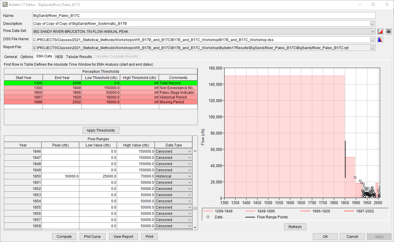
Now, information needs to be added to the Perception Thresholds table to account for the NEB and PSI. Two perception thresholds will need to be used since the perceivable range of flows during these periods are markedly different (one for the NEB and one for the PSI). One way to interpret the NEB data would be to enter a perception threshold of [150,000 – inf] for the period between 1300 – 1849. For the PSI, one could enter a perception threshold of [50000 – inf] for the period between 1850 – 1896, as shown in the following figure.
However, this is by no means the only way to interpret the available data.

- Use the Comments column to provide an adequate descriptive note for each row.
Utilize the Right Click | Sort by Start Year function to sort the rows.
- Once all of the information has been entered to the Perception Thresholds table, click Apply Thresholds. This will fill out the Flow Ranges table with the complementary information.
Now, the PSI (i.e. discrete event) needs to be added to the Flow Ranges table.
- Enter a Peak, Low, and High flow value for the PSI event. This information, along with the year in which you think the PSI event occurred, should be entered based upon your interpretation of the paleoflood data presented earlier. Don't forget to change that year's Data Type to Historical in the last column.
It is possible that your interpretation of the age and magnitude(s) of the PSI event will differ from others.
- Ensure that the Flow Ranges table contains a low and high value for every single year in the analysis period.
- A possible interpretation of the paleoflood data is shown within the following figure.
- Click Compute.
Analyze Results
- Click Plot Curve. This will result in the computed curve, 5- and 95-percent confidence limits, and observed events being plotted.
- Close the computed curve window.
- Move to the Tabular Results Note the computed curve, 5-, and 95-percent confidence limits for all of the desired frequency ordinates, the moments/parameters of the Log Pearson Type III fit to the data, and other data related to the analysis.
Question: How do the Log Pearson Type III parameters (mean, standard deviation, and skew) compare between the BigSandyRiver_Paleo_B17C and BigSandyRiver_Historical_B17C analyses? Why are they different? How do these differences affect the 1-percent chance exceedance flow rate? How do these differences affect your estimates of peak flow for rarer exceedance probabilities (e.g., 0.01-percent chance exceedance)? How did the ERL estimate change between the two analyses?
The mean and standard deviation for the BigSandyRiver_Paleo_B17C analysis are slightly larger than those computed within the BigSandyRiver_Historical_B17C analysis. However, the computed at-site skew for the BigSandyRiver_Paleo_B17C analysis is much larger. This affects the flow rates for smaller exceedance probabilities.
The BigSandyRiver_Paleo_B17C computed 1-percent chance exceedance flow rate is approximately 3000 cfs greater than the BigSandyRiver_Historical_B17C analysis. Also, the differences for much rarer exceedance probabilities are much greater due to the increase in skew, as shown in the following figure.
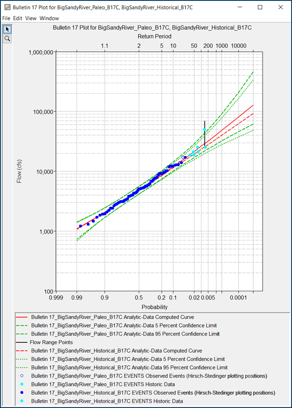
The ERL for the BigSandyRiver_Paleo_B17C analysis increased by approximately 136 years. This translates to a substantial reduction in uncertainty in these results due to the inclusion of paleoflood data.
Question: Fill out the following tables.
If you have not done so already, you will need to add Output Ordinates to the BigSandyRiver_Historical_B17C analysis to complete the Paleoflood vs Historical Flow Frequency Information table.
Paleoflood vs Historical Analysis Statistics
Statistic | Historical | Paleoflood |
|---|---|---|
Systematic Events |
|
|
Historic Period (years) |
|
|
Mean | ||
Standard Deviation | ||
Station Skew | ||
Adopted Skew |
Paleoflood vs Historical Flow Frequency Information
Recurrence Interval (years) | Annual Chance Exceedance (%) | Peak Flow (cfs): | |
|---|---|---|---|
Historical | Paleoflood | ||
100000 | 0.001 | ||
10000 | 0.01 | ||
1000 | 0.1 | ||
500 | 0.2 | ||
200 | 0.5 | ||
100 | 1 | ||
50 | 2 | ||
20 | 5 | ||
10 | 10 | ||
The quantiles noted above have been rounded.
Statistic | Historical | Paleoflood |
|---|---|---|
Systematic Events | 65 | 65 |
Historic Period (years) | 113 | 710 |
Mean | 3.685 | 3.692 |
Standard Deviation | 0.289 | 0.298 |
Station Skew | 0.064 | 0.171 |
Recurrence Interval (years) | Annual Chance Exceedance (%) | Peak Flow (cfs): | |
|---|---|---|---|
Historical | Paleoflood | ||
100000 | 0.001 | 93130 | 128500 |
10000 | 0.01 | 62780 | 80990 |
1000 | 0.1 | 40090 | 48320 |
500 | 0.2 | 34500 | 40750 |
200 | 0.5 | 27890 | 32060 |
100 | 1 | 23420 | 26370 |
50 | 2 | 19370 | 21370 |
20 | 5 | 14610 | 15680 |
10 | 10 | 11390 | 11970 |
Question: Try adjusting only the inferred ages of the NEB and PSI. How do these changes affect the LPIII distribution?
Try adjusting the age of the NEB to be older than you originally assumed without adjusting the magnitude. Then, try adjusting the age of the NEB to be younger than you originally assumed without adjusting the magnitude. How do these changes affect the computations?
The mean and standard deviation do not change all that much. Also, the skew coefficient varies between approximately 0.177 (for the shortest inference of age) and approximately 0.147 (for the oldest inference of age). This results in only slight changes to the flow-frequency curve, even for extremely rare exceedance probabilities, as shown in the figure below. The results of this sensitivity analysis demonstrate a relative insensitivity to the age inference of both the PSI and NEB.
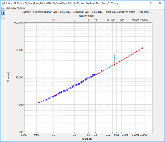
Question: Try adjusting only the inferred magnitudes of the NEB and PSI (i.e. flow values). How do these changes affect the LPIII distribution?
Similar to adjusting the ages of the NEB and PSI, the mean and standard deviation do not change to a large degree. However, the skew coefficient varies between approximately 0.105 (for the smallest inference of PSI and NEB magnitudes) and approximately 0.184 (for the largest inference of PSI and NEB magnitudes). This results in noticeable differences to the flow-frequency curve for extremely rare exceedance probabilities, as shown in the following figure.
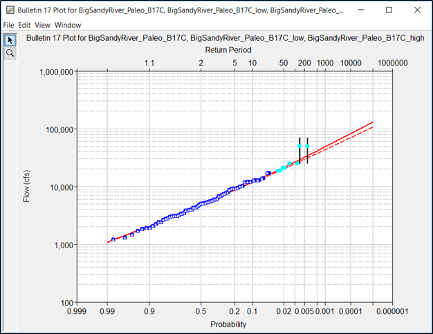
The plotting position of the PSI event (represented by a flow range in the plot above) has a different x-axis position (i.e. plotting position) within the “low” analysis. This is due to the fact that the magnitude of the PSI event for this analysis is greater than the magnitude of the perception threshold causing it to plot to the right (i.e. less frequent). However, remember that the plotting positions do not affect the computed curve.
Conclusion
This concludes the Using Bulletin 17C Methodology within HEC-SSP workshop. If time allows, continue to Optional Task. Bulletin 17B | Systematic Record.
