Download PDF
Download page Task 3. Bulletin 17C | Systematic Record + Historical Information.
Task 3. Bulletin 17C | Systematic Record + Historical Information
Return to Task 2. Bulletin 17C | Systematic Record.
Create a New Bulletin 17 Analysis
Historical event information can be used to both add important information and place the systematic information into a longer context. Three historical events occurring in 1897, 1919, and 1926 are available for the Big Sandy River at Bruceton, TN gaging station. This information can be incorporated within a Bulletin 17 analysis.
- To begin, select Analysis | New | Bulletin 17 Analysis.
- Name the new analysis “BigSandyRiver_Historical_B17C” and add an adequate description.
- Select the “BigSandyRiver” data set.
- Select “17C EMA” within the Method for Computing Statistics and Confidence Limits panel.
- Utilize the default selections of Use Station Skew, Multiple Grubbs-Beck low outlier test, and Hirsch/Stedinger plotting position.
Input EMA Data
- Move to the EMA Data tab.
When using Bulletin 17C procedures within HEC-SSP, modifications to the time window and historical information are made on the EMA Data tab. The first row of the Perception Thresholds table controls the time window of the entire analysis. Since we’d like to include historical information dating back to 1897, the first row of the Perception Thresholds table needs to be modified.
- Change the first row in the Perception Thresholds table so that the analysis spans 1897 through 2009. The low and high perception thresholds for this first row should be left at 0 and “inf”.
- In the Flow Ranges table, add the historic event information for 1897.
- Enter 25000 for the Peak.
- Use the drop down Data Type menu to set this year to Historical.
- Also set the Low and High Values to 25000.
Question: What does a Low and High value that are equivalent imply about the uncertainty in the peak flow rate for this event?
This implies that there is no uncertainty with the observed peak flow rate (which may or may not be true in all cases).
- In a similar manner, add the historic event information for the 1919 and 1926.
- Enter 21000 for the Peak, Low, and High values in 1919.
- Enter 18500 for the Peak, Low, and High values in 1926.
- Ensure that the Data Type for both of these years is set to Historical.
Now, information needs to be added to the Perception Thresholds table to account for the missing periods between 1898-1918, 1920-1925, 1927-1929, and 1988-2002. A single perception threshold can be used since the perceivable range of flows did not change during that time frame. A reasonable choice would be to utilize the smallest historical event that occurred during the time frame in question. This assumes that had an event similar in magnitude to the 1926 event occurred, it would have been noted. ***However, this is by no means the only way to interpret the available data.***
- Enter “1897”, “1929”, “18000”, and “inf” for the Start Year, End Year, Low Threshold, and High Threshold in the second row.
- Enter “1988”, “2002”, “18000”, and “inf” for the Start Year, End Year, Low Threshold, and High Threshold in the third row.
You can utilize the Right Click | Sort by Start Year option to automatically sort the contents of the Perception Thresholds
Question: Similar to the previous analysis which used only Systematic data, what does the use of this perception threshold imply about the missing periods?
The use of these perception thresholds assumes that had a peak flow rate occurred in excess of 18000 cfs during any of these missing periods, it would have been observed and recorded. This is true of both the 1897 - 1929 and 1988 - 2002 periods.
- Use the Comments column to provide an adequate descriptive note for each row.
- The Perception Thresholds table should resemble the following figure.

- Once all of the information has been entered to the Perception Thresholds table, click Apply Thresholds. This will fill out the Flow Ranges table with the complementary information.
- Ensure that the Flow Ranges table contains a low and high value for every single year in the analysis period.
- The completed EMA Data tab should resemble the following figure.

- Click Compute.
Analyze Results
- Click Plot Curve. This will result in the computed curve, 5- and 95-percent confidence limits, and observed events being plotted.
- Close the computed curve window.
- Move to the Tabular Results Note the computed curve, 5-, and 95-percent confidence limits for all of the desired frequency ordinates, the moments/parameters of the Log Pearson Type III fit to the data, and other data related to the analysis.
Question: How did the inclusion of additional historical information affect the Log Pearson Type III parameters (mean, standard deviation, and skew)? How does this affect the 1-percent chance exceedance flow rate? How did this affect the computed ERL?
Multiple analyses can be compared in many ways. For instance, the results from two or more analyses can be plotted together by first selecting the analyses in the tree and clicking Results | Graph. Also, additional information can be compared for multiple analyses by selecting them and clicking Results | Summary Report.
The mean, standard deviation, and skew magnitudes are all larger when historical information is included. The BigSandyRiver_Historical_B17C 1/100 AEP flow rate is approximately 4500 cfs larger than the BigSandyRiver_Systematic_B17C results, as shown below.
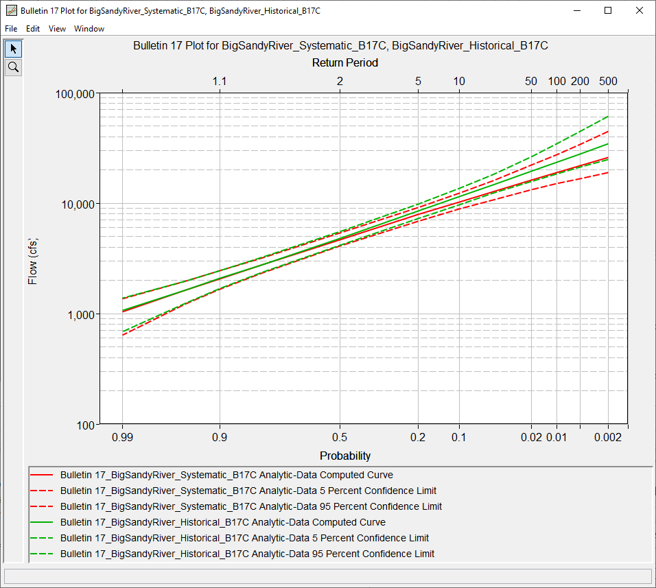
The ERL for the BigSandyRiver_Historical_B17C analysis is approximately 23 years larger than the BigSandyRiver_Systematic_B17C analysis. Thus, using a perception threshold of [0 - 18000 cfs] for the period spanning 1897 - 1929 added 23 years' worth of information to the analysis. This translates to a reduction in uncertainty in these results due to the inclusion of historical data.
Question: Observe and record the following information.
Copy the following tables and fill in using results from your own simulations.
Statistic | Systematic | Historical |
|---|---|---|
Systematic Events |
|
|
Historic Period (years) |
|
|
Mean | ||
Standard Deviation | ||
Station Skew | ||
Adopted Skew |
Recurrence Interval | Annual Chance Exceedance | Peak Flow (cfs): | |
|---|---|---|---|
Systematic | Historical | ||
500 | 0.2 | ||
200 | 0.5 | ||
100 | 1 | ||
50 | 2 | ||
20 | 5 | ||
10 | 10 | ||
The quantiles noted below have been rounded.
Statistic | Systematic | Historical |
|---|---|---|
Systematic Events | 65 | 65 |
Historic Period (years) | 80 | 113 |
Mean | 3.665 | 3.685 |
Standard Deviation | 0.271 | 0.289 |
Station Skew | -0.090 | 0.064 |
Recurrence Interval | Annual Chance Exceedance | Peak Flow (cfs): | |
|---|---|---|---|
Systematic | Historical | ||
500 | 0.2 | 26030 | 34500 |
200 | 0.5 | 21890 | 27890 |
100 | 1 | 18950 | 23420 |
50 | 2 | 16170 | 19370 |
20 | 5 | 12710 | 14610 |
10 | 10 | 10230 | 11390 |
Continue to Task 4. Bulletin 17C | Systematic Record + Historical Information + Paleoflood Information.