Part 1 - New Hydrologic Sampler Alternative
Objective
Your objective in Part 1 is to create and define a new Hydrologic Sampler alternative designed for the Russian River example study. Specifically, Part 1 guides you through creating a new Hydrologic Sampler alternative and entering the information required for generating basin-wide precipitation events in the Russian River basin, based on the Basin-Average frequency curve method.
Part 1.0 – Create the New Hydrologic Sampler Alternative
1. Open the HEC-WAT software. From the downloaded folder, open the HEC-WAT watershed called "sty". In this watershed, a Hydrologic Sampler alternative already exists and is used in the Existing FRA simulation, but we will create a new Hydrologic Sampler alternative to replace the existing Hydrologic Sampling alternative used in the simulation.
2. Create a new Hydrologic Samper alternative from the Study Tree. Expand the Models tree (click ![]() ), right-click the Hydrologic Sampling model, and click New from the shortcut menu.
), right-click the Hydrologic Sampling model, and click New from the shortcut menu.
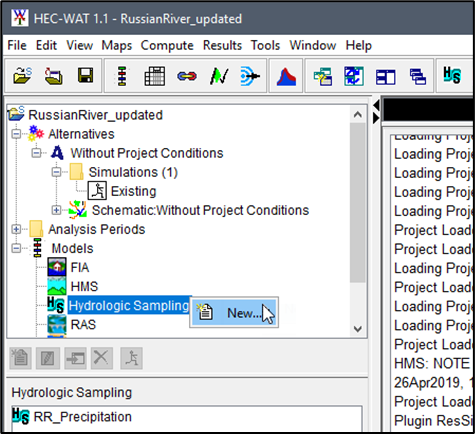
Alternatively, create a new alternative, from the HEC-WAT main window, click Edit | Hydrologic Sampling | New.
Either way the Create New Hydrologic Sampling Alternative dialog opens.
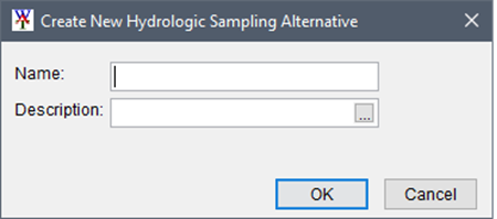
3. From the Create New Hydrologic Sampling Alternative dialog, provide the Name for the new alternative “RR_Precip,” (a description can be entered) and click OK. The Hydrologic Sampling Editor will open.

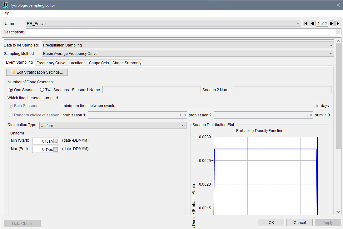
4. Now we need to select the correct data type and method. From the Data to be Sampled and Sampling Method dropdown lists select Precipitation Sampling and Basin Average Frequency Curve, respectively. The Editor updates.
Part 1.1 – Enter the Season Distribution
The season distribution describes when events are likely to occur, and will be randomly sampled to choose a date for each generated event. A histogram of when the annual maximum events occurred is shown in a previous figure, with a bar for each half month through the year. Note that events occur only in the winter, primarily between December and February.
We’ll be using an empirical probability distribution to capture this flood season distribution in the Hydrologic Sampling Editor.
- Note that the Hydrologic Sampling Editor has opened to the Event Sampling tab.
- From the Number of Flood Seasons section, keep One Season selected.

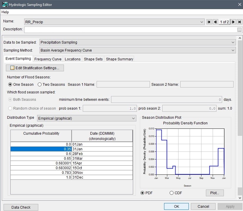
1. From the Distribution Type dropdown list, select the Empirical (graphical) distribution for the flood season. Note the Empirical (graphical) distribution table added to the Editor.
2. Open the spreadsheet “Workshop_inputs.xlsx” and navigate to the Season Distribution Select the data in cells B3:C10, copy (Ctrl+C).
Return to the Hydrologic Sampling Editor and in the Empirical (graphical) distribution table select the upper left cell (in Cumulative Probability column) and paste (Ctrl+V) the copied data.
The probabilities and dates should appear in the distribution table. Double-click any of the values to update the PDF plot.
- Click Apply. The Editor should look like the figure below. (Note, The figure below has been modified to reduce the size of the duration plot and, therefore, the overall size of the figure.)
Part 1.2 – Define the Basin Average Frequency Curve
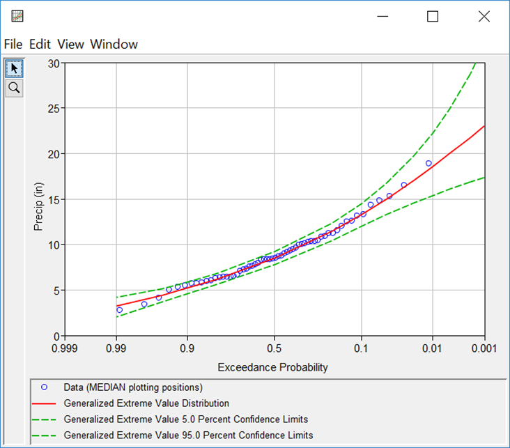
A precip-frequency curve was estimated by a GEV distribution using the 60 years of annual maximum 8-day precipitation accumulations, and is shown in the figure below. This is the distribution we’ll be using to generate random basin-average precipitation depths for each event.
1. In the Hydrologic Sampling Editor, select the Frequency Curve tab. Complete the following steps to enter the duration sampling, watershed name, time window, and frequency curve duration information.
- For the Duration Sampling Options and Time Window Option at the top, keep all default selections. (Single Duration radio button, Watershed 1 from the dropdown, and Basin Average radio button.)
2. In the Duration Selection panel, ensure the default selection Days appears on the dropdown list, and in the textbox enter 8 to set the duration as 8 days. This specifies that the frequency curve we’re using is for 8-day precipitation depth.
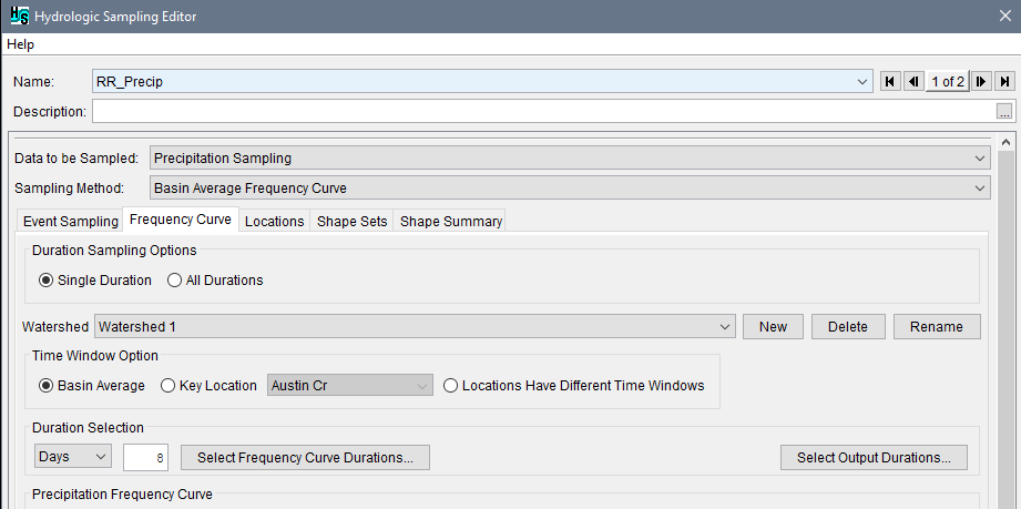
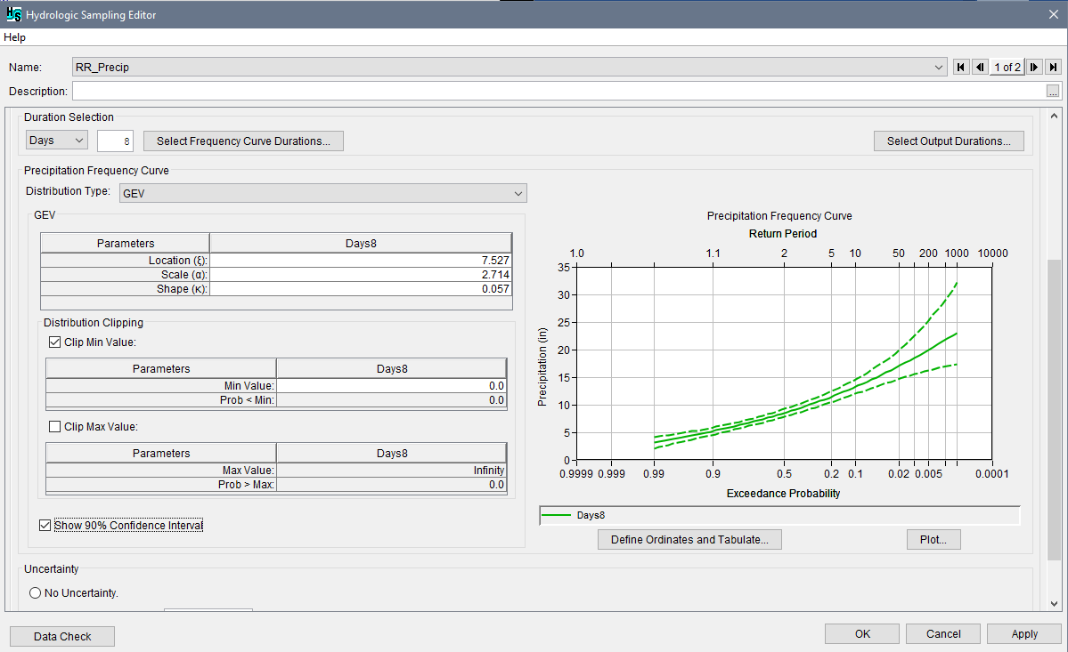
3. Next, the precipitation frequency curve must be defined. Moving down to the Precipitation Frequency Curve panel, from the Distribution Type list select GEV. Parameters are required for location, shape and scale.
4. Navigate to still open Excel spreadsheet “Workshop_inputs.xlsx,” and select the GEV parameters Select the values listed for location, scale and shape, and copy the three values. Navigate back to the Hydrologic Sampling Editor and for the GEV distribution table, select all 3 cells and paste the parameter duration values for location, scale and shape. Note, the frequency curve plot updates automatically.
5. Next, From the Distribution Clipping panel, check the checkbox to enable Clip Min Value and enter 0.0 as the Min Value.
6. Last, we will enter the uncertainty about the frequency curve. From the Uncertainty panel, keep the default selection of years of record, and enter 60 in the textbox. This uncertainty is chosen because the frequency curve is based on 60 years of data.
- Click Apply.
7. To update the frequency curve plot to view the uncertainty about the curve, from the GEV panel, check the checkbox for Show 90% Confidence Interval, a Computation Warning window will appear, click OK to close to window, then click Apply. The frequency curve confidence intervals and the Editor should look like the figure below.
Part 1.3 – Enter the Hyetograph Locations
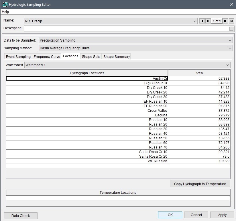
1. In the Hydrologic Sampling Editor, select the Locations tab. This Tab is where we enter the sub-basins of the HEC-HMS model alternative, (MCA)Russian River FRA, and their drainage areas. The Hydrologic Sampler will create a hyetograph for each sub-basin for each event generated.
- From the Watershed dropdown list, keep the default selection of Watershed 1.
2. Navigate to still open Excel spreadsheet “Workshop_inputs.xlsx,” and select the Locations Copy the location names and areas from the spreadsheet. Navigate back to the Hydrologic Sampling Editor, select the upper left cell in the table, and paste the copied information.
3. Click Apply. The Editor should look like the figure below.
Part 1.4 – Define Shape Sets
Select DSS Pathname
1. In the Hydrologic Sampling Editor, select the Shape Sets tab. The shape sets must be created one at a time, and populated by a DSS record for each location. To create a new shape set, click the New Set button to open the Create New Shape Set dialog.
2. Enter the Name of the set as “Dec_1955,” and click OK. Note, in the Shape Sets tab the Hyetograph Time-Series table updates with Location names for Watershed 1 filled in (according to the information entered in the Locations tab) for setting the DSS pathnames. At this point we will keep the default values for the shape set Exceedance probability filter and Weight information; instead, these values will be modified for all shape sets in Part 1.6.
3. Move to the Hyetograph Time-Series table and select a cell in the first row.
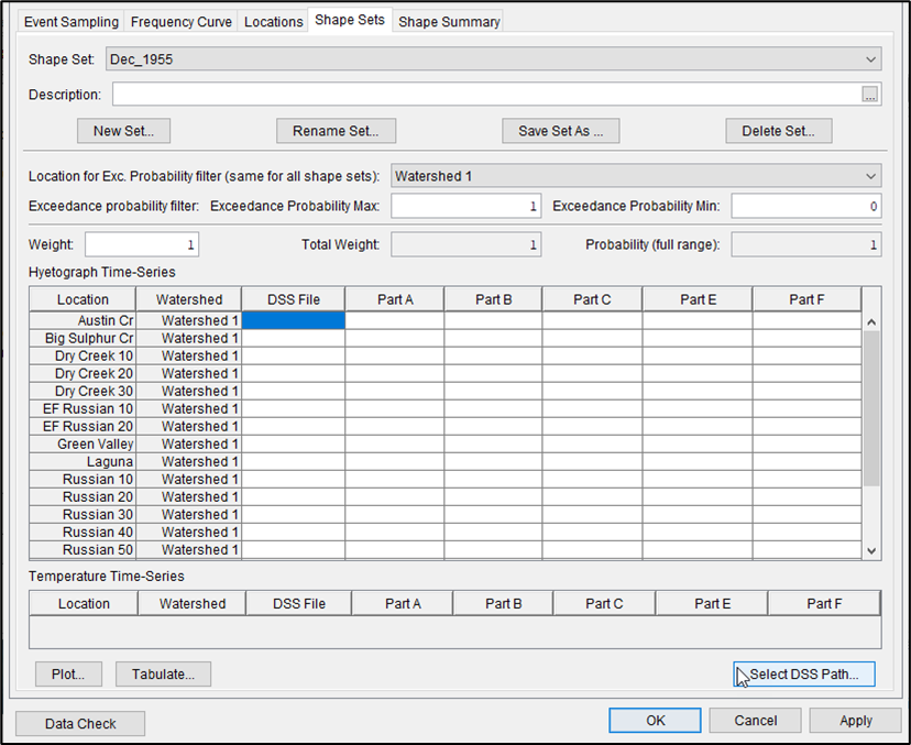
Click the Select DSS Path button, and an HEC-DSSVue pathname selection window opens.

4. From the HEC-DSSVue toolbar click ![]() , and an Open HEC-DSS File browser window opens. Navigate to the shared subdirectory, in the HEC-WAT study folder, select “Dec 1955 shapeset.dss” and click Open. The HEC-DSSVue window will update with the selected DSS file.
, and an Open HEC-DSS File browser window opens. Navigate to the shared subdirectory, in the HEC-WAT study folder, select “Dec 1955 shapeset.dss” and click Open. The HEC-DSSVue window will update with the selected DSS file.
- Move the HEC-DSSVue window so that you can see both windows (Hydrologic Sampling Editor and the HEC-DSSVue window) simultaneously (e.g., side-by-side).
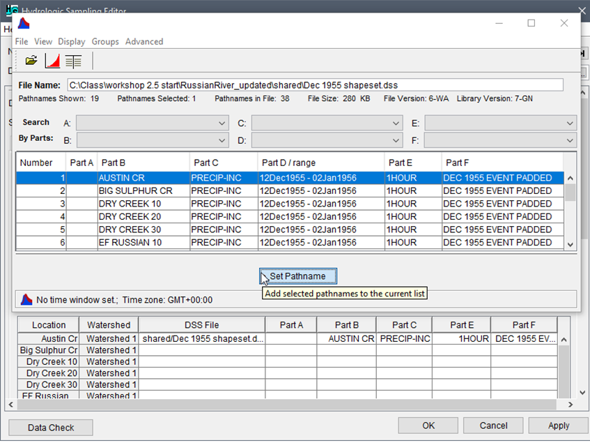
5. In the HEC-DSSVue window, select the HEC-DSS record with B-part that matches the current row’s Location name listed in the Hydrologic Sampling Editor (which will be “AUSTIN CR” for the first row) and click the Set Pathname button.
- Note that the table in the Hydrologic Sampling Editor has been populated by the pathname parts.
6. Return to the Hydrologic Sampling Editor, and select the next row in the table, for “Big Sulphur Cr.” Return to the HEC-DSSVue window, select the record for “BIG SULPHUR CR” and again click the Set Pathname button.
7. Continue and complete this shape set using the copy and paste method (see Step 8, below). Close the HEC-DSSVue set pathname window.
Copy and Paste DSS Pathname
It is also possible to fill in the Hyetograph Time-Series table by pasting the DSS pathnames copied from a spreadsheet. We will complete shape set Dec_1955 and create and complete shape set Dec_1964 by copying the Hyetograph Time-Series table from the open “workshop_inputs.xlsx” spreadsheet, using the pathnames provided in the Shape Sets sheet.
8. To complete Dec_1955, navigate to the “workshop 2.4 inputs.xlsx” spreadsheet, find the pathnames for the "December 1955" event, select and copy cells A3:F21. Return to the Hydrologic Sampling Editor, select all the cells in the table (all rows, beginning in the DSS column and spanning to Part F column) and paste (Ctrl+V).
- NOTE: make sure that you always ensure that you’ve scrolled to the top of the table all the way to the bottom to select all rows before pasting. In other words, the paste command only works for cells considered active, and only selected cells in the Hyetograph Time-Series table are considered active.
- Click Apply. Click the Plot button to see the linked records. Close the plot.
9. From the Shape Sets tab, create another new shape set by clicking the New Set button, and the Create New Shape Set dialog opens.
10. Enter the Name of the set as “Dec_1964,” and click OK. Keep the default values for the shape set the Exceedance probability filter and Weight information; recall, these values will be modified for all shape sets in Part 1.6.
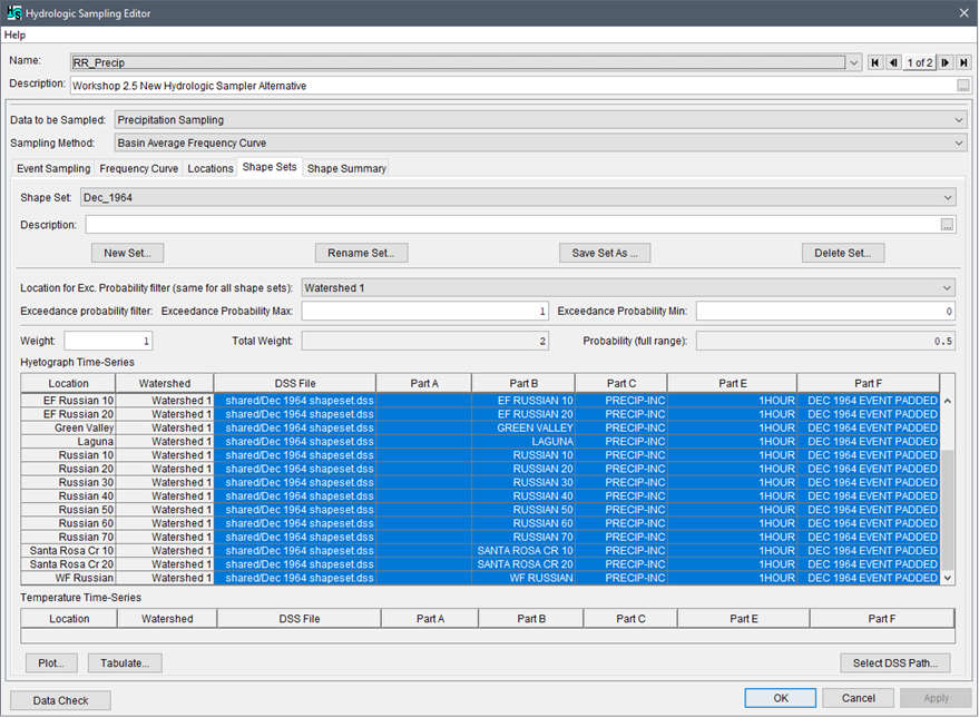
11. Navigate to the “workshop_inputs.xlsx” spreadsheet, find the pathnames for the "December 1964" event, select and copy cells A25:F43. Return to the Hydrologic Sampling Editor, and select all the cells in the table (all rows, beginning in the DSS column and spanning to Part F column) and paste (Ctrl+V).
- Click the Plot button to see the linked records. Close the plot. Click Apply. The Editor should look like figure below.
Part 1.5 – Enter Shape Set Ranges
1. From the Hydrologic Sampling Editor, navigate to the Shape Set Summary tab. As previously explained, we have not yet specified limited ranges of exceedance probability for use of these shapes (as set by default, the minimum is 0.0 and maximum is 1.0), so any shape may be chosen for any event. Also the weights are all 1.0, so the probability of each event being chosen is 0.5.
2. Enter new exceedance ranges for the following shape sets:
- For Dec_1955, change the value for Exceedance Probability Maximum to 0.1.
- For Dec_1964, change the Exceedance Probability Minimum to 0.1.
3. Click Apply. The Editor should look like the figure below.
Note
The figure below shows which shapes are available for which exceedance probability ranges in the plot below the table. Also note that the probability column in the table now shows those first shape sets less likely to be chosen, as that set can only be chosen in a smaller probability range.

Part 1.6 – Data Check
1. Click the Data Check button. If all of the above steps have been followed correctly, you should get a Message window saying “No data consistency errors.” If not, the Message window will list instances where information was not provided properly for the RR_Precip model alternative. Review those instances to find the errors, and repeat those steps then use the Data Check to re assess the RR_Precip model alternative.
2. Close the Hydrologic Sampling Editor by clicking OK.
3. Save the HEC-WAT study (from the File menu click Save Study, or from the HEC-WAT toolbar click ![]() ).
).