Reservoir Stratification

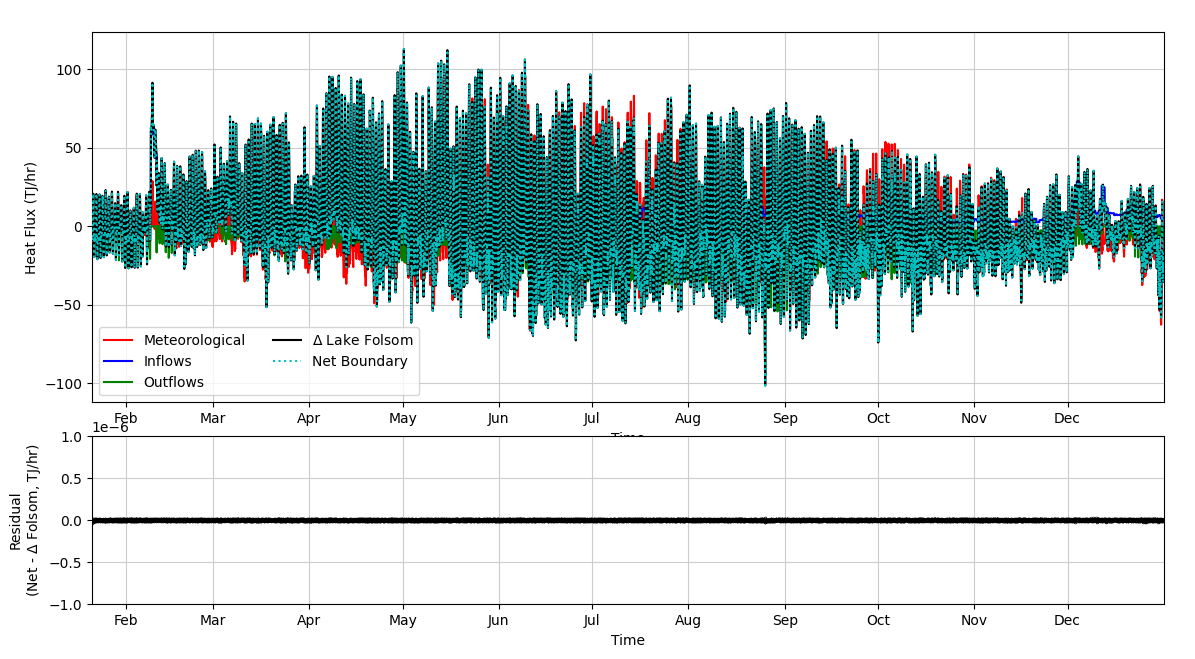
A test simulation was performed using the full American River network (see Transport of a Conservative Constituent), with water temperature as the only active constituent. The purpose of this test simulation was to examine the model-calculated heat budget terms on Lake Folsom, and verify the conservation of energy equation.

The simulation period was calendar year 2014. Lake Folsom was given an isothermal initial condition of 10°C. Inflows, reservoir operations, boundary conditions, and meteorological data were based on observed data for the watershed. An example inflow boundary temperature record and the meteorological data records are shown below.

The contour plot below shows the setup and breakdown of stratification in the reservoir through the simulation period.

In order to verify the heat budget calculations, the heat content of the reservoir was calculated as:

$\begin{array}{l}\displaystyle H_{\textrm{Folsom}} = \rho \, C_p \, \sum_k \, V_k \, T_k\end{array}$

where

$\begin{array}{l}H_{\textrm{Folsom}}\end{array}$ is the heat content of Lake Folsom (J),
$\begin{array}{l}V_k\end{array}$ is the computational layer volume (m³),
$\begin{array}{l}T_k\end{array}$ is the temperature of the layer (°C),
$\begin{array}{l}\rho\end{array}$ is the water density (assumed = 1000 kg/m³), and
$\begin{array}{l}C_p\end{array}$ is the specific heat of water (assumed = 4186 J/kg/°C).

The change in heat content from time step to time step ( $\begin{array}{l}\Delta H_{\textrm{Folsom}}\end{array}$ ) was compared to the net boundary heat fluxes for the reservoir. These include inflow, outflow, and meteorological fluxes (shortwave radiation, longwave radiation, evaporative, and sensible). Heat fluxes associated with inflows and outflows ( $\begin{array}{l}F_Q\end{array}$ ) were calculated as:

$\begin{array}{l}\displaystyle F_Q = Q \, \rho \, C_p \, T_Q\end{array}$

where

$\begin{array}{l}Q\end{array}$ is the inflow or outflow magnitude (m³/s), and
$\begin{array}{l}T_Q\end{array}$ is the temperature of the flow (°C).

Net meteorological fluxes ( $\begin{array}{l}F_{met}\end{array}$ ) were calculated by using the heat fluxes output from the Water Temperature Simulation Module (WTSM) (in W/m²) and multiplying by the layer top area ( $\begin{array}{l}A_k\end{array}$ ). For the surface layer, the surface area of the reservoir was used; for all deeper layers, the area was the top area of each computational layer.

$\begin{array}{l}\displaystyle F_{met} = \sum_k \, \left( q_{sw,k} + q_{atm,k} - q_{b,k} + q_{h,k} - q_{l,k} + q_{sed,k} \right) A_k\end{array}$

Longwave ( $\begin{array}{l}q_{sw}, q_{atm}\end{array}$ ), sensible ( $\begin{array}{l}q_h\end{array}$ ), and latent ( $\begin{array}{l}q_l\end{array}$ ) heat fluxes were only non-zero in the surface layer.

To check closure of the heat budget, the residual between the change in heat in Lake Folsom and the sum of the boundary heat fluxes was calculated as:

$\begin{array}{l}\displaystyle \textrm{Residual} = \Delta H_{\textrm{Folsom}} - (F_{Qin} - F_{Qout} + F_{met}) \Delta t\end{array}$

where $\begin{array}{l}\Delta t\end{array}$ is the computational time step (sec).

A plot of the hourly heat fluxes is shown below. The full period is first shown, and then a few days in July are given to see the diurnal variations. Below each heat flux plot is the residual time series. Residuals were approximately 1 x 10^-8, indicating a successful closure of the heat budget.

A plot of the individual terms in the heat budget is shown below for a week in early July.