Download PDF
Download page Transport of a Conservative Constituent.
Transport of a Conservative Constituent
A series of test simulations was used to document the WQ Engine's mass conservation properties. The simulations used the American River watershed, which was previously set up and calibrated to hydrology and water temperature (USBR, 2024). This watershed was chosen because it is a relatively simple watershed (containing two reservoirs, and six reach segments), but still contains complex reservoir operations, diversions and local inflows. Datasets were previously compiled to simulate any period of time between 2001 and 2020.
Two geometries were used in the testing:
1) The full lower American watershed, containing Lake Folsom, Lake Natoma, and the lower American River, and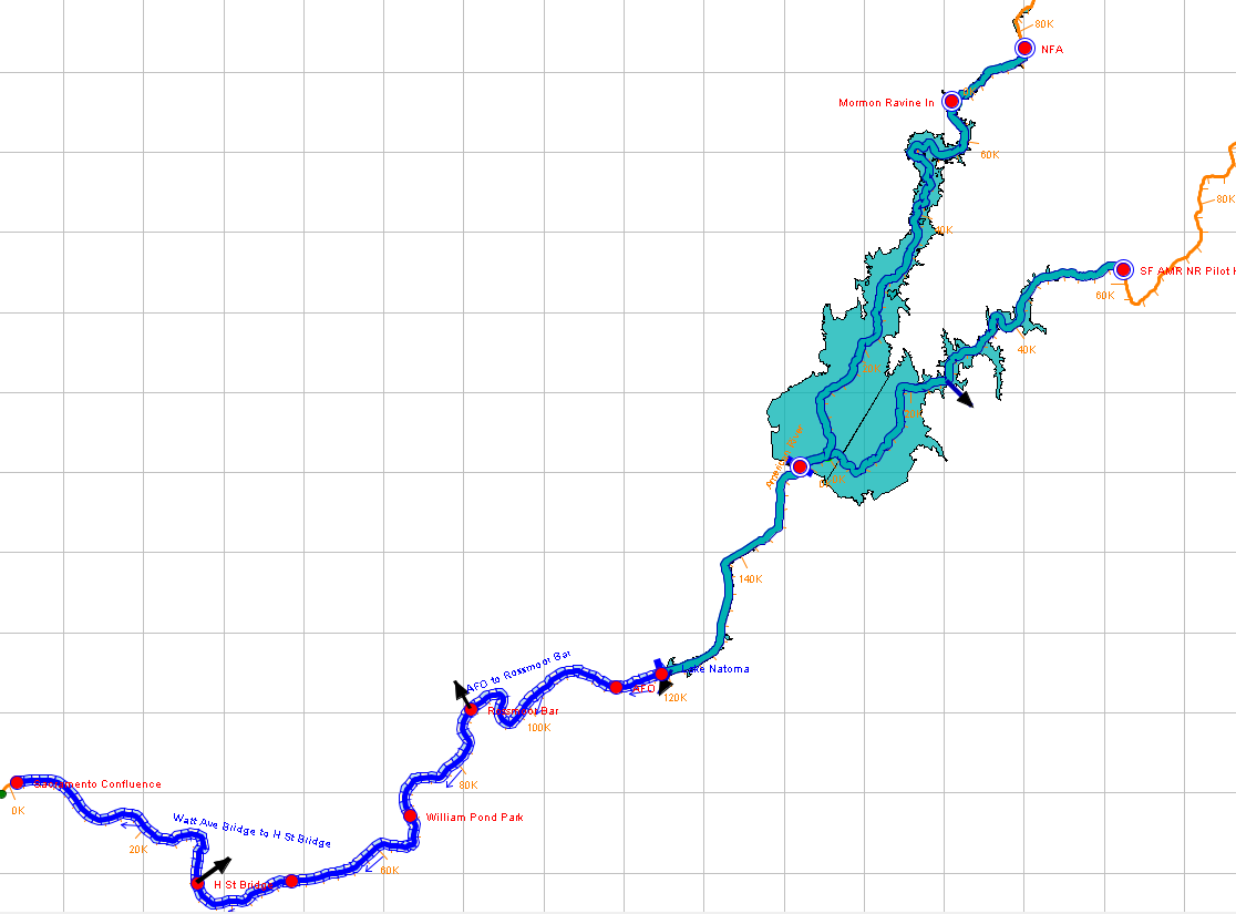
2) The lower American River only, starting at the outlet of Lake Natoma.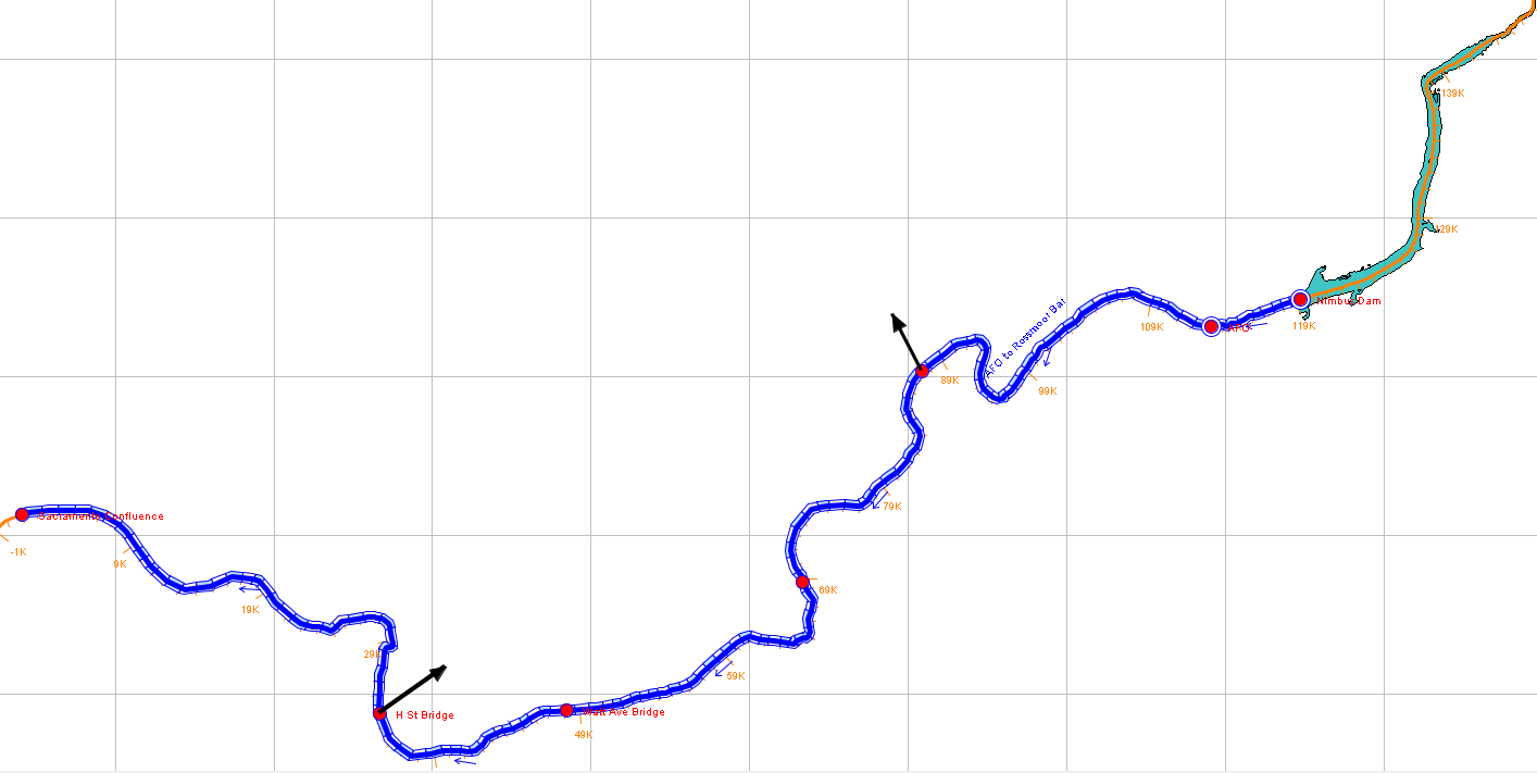
A conservative constituent was added to the existing water temperature model. Simulations were performed with both the water temperature and the conservative constituent active. The purpose of these tests was to measure the conservation of mass properties of the tracer for different flow conditions, computational assumptions, and reach routing methods. The inclusion of temperature in the simulations ensured that tracer inflows and outflows to the reservoirs occurred over a range of thermal stratification conditions.
Zero Concentration Test
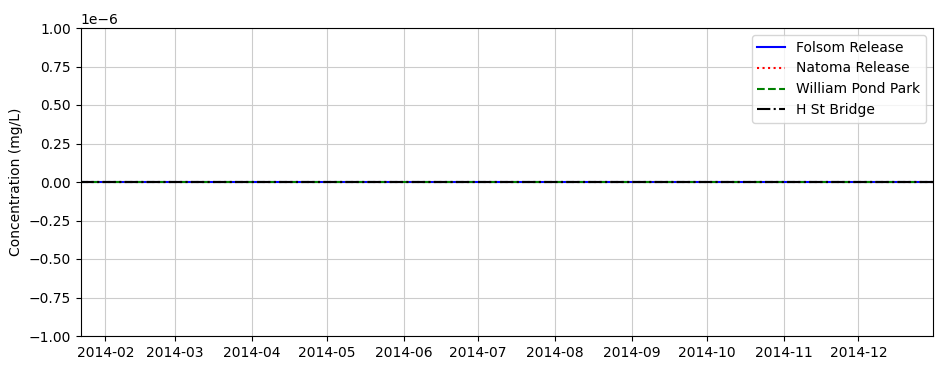
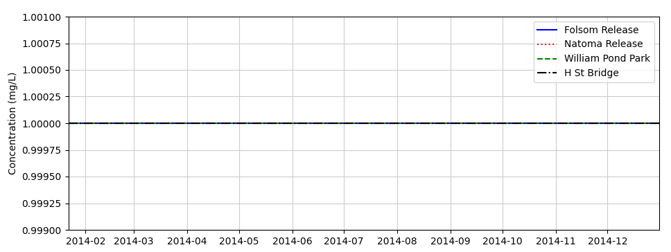
The first and simplest test used the full watershed geometry, an initial condition of zero concentration everywhere, and boundary concentrations of zero. A representative year (2014) was chosen for the simulation. A check was made to ensure the model maintained concentrations that were identically zero throughout the simulation. Shown below is the time series of constituent concentrations at the outflows from Folsom and Natoma, as well as two locations downstream on the American River. This simulation included all of the normal reservoir operations, diversions and local inflows, and unsteady flow in the system.
Constant Concentration Test
A second simple test was performed with the initial constituent concentrations of 1.0 mg/L everywhere and 1.0 mg/L for all boundary concentration inflows. A check was made to ensure the model maintained concentrations of 1.0 mg/L throughout the simulation.
Tracer Pulse Test
This test case used the river-only geometry and was intended to highlight the mass conservation and travel time tradeoffs between different computational options.
A pulse of a conservative scalar was input as a boundary condition on the upstream end of the river network. The pulse was one hour in duration and had a concentration of 100 mg/L. The remainder of the upstream boundary time series had a concentration of zero. The pulse of the conservative scalar was tracked as it moved downstream through the system, and its transport was compared against the analytical solution to the 1D wave equation.
The 1D wave equation describes the transport of a dissolved constituent traveling with the flow, absent of any dispersion or source/sink transformations:
| \frac{\partial C}{\partial t} + v \frac{\partial C}{\partial x} = 0 |
where v is the stream velocity. The analytical solution to this equation is C(x,t) = C_o(x - vt), where C(x,0) = C_o(x) is the initial condition. The solution implies that the initial concentration profile is translated downstream without modification.
To set up a test case for inspection of travel times and comparison with the wave equation solution, a modified version of the HEC-RAS steady flow file was input to the lower American River model. Each cross-section was given a velocity of 0.5 ft/s at every flow in the steady flow table. User-input dispersion coefficients were set to zero for all river segments, and all water diversions were negated. A three day simulation using hourly time steps was performed to transport the tracer pulse down the approximately 22 mile stretch of river.
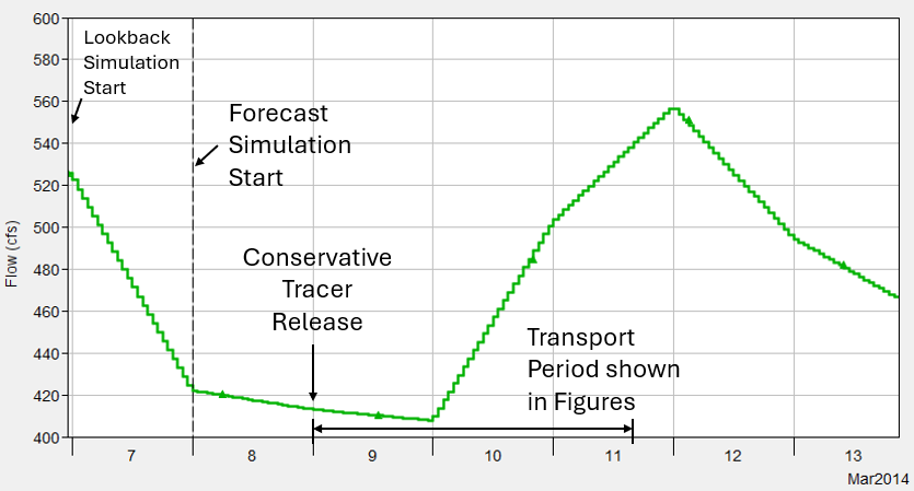
River flow in the simulation was unsteady. The figure below shows the boundary flows entering the river from the Lake Natoma dam release. Annotations on the plot show the simulation lookback time, the simulation start time, the tracer release time, and the period over which the tracer was tracked on its virtual journey down the American River. Null routing was used as a hydrologic routing method for all of the reach segments. Note that, even though the flow rate is unsteady in time, the modified RAS steady flow file meant that the cross-sectional velocities that were passed to the WQ Engine from ResSim were 0.5 ft/s regardless of flow.
First Order Transport
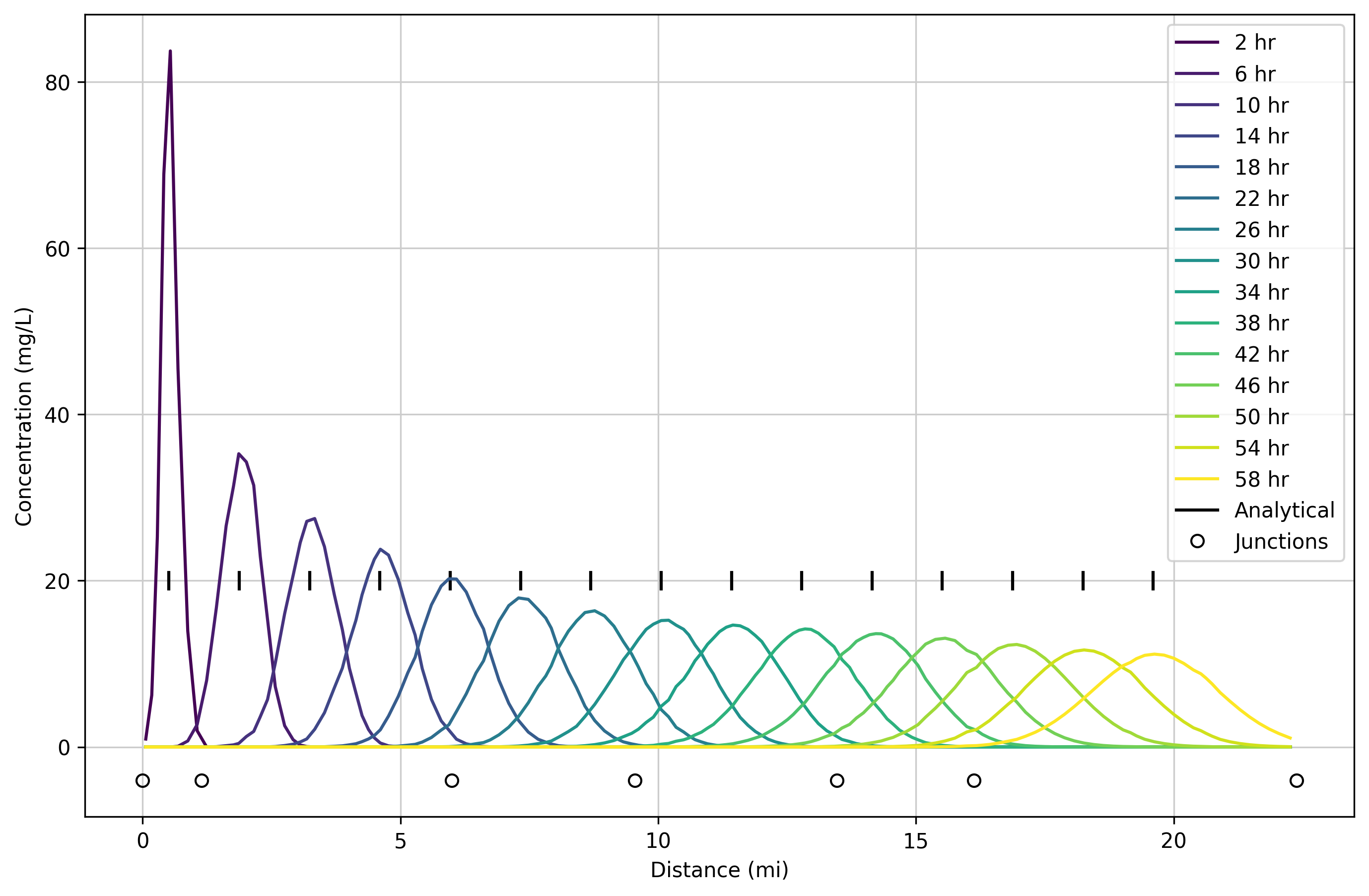
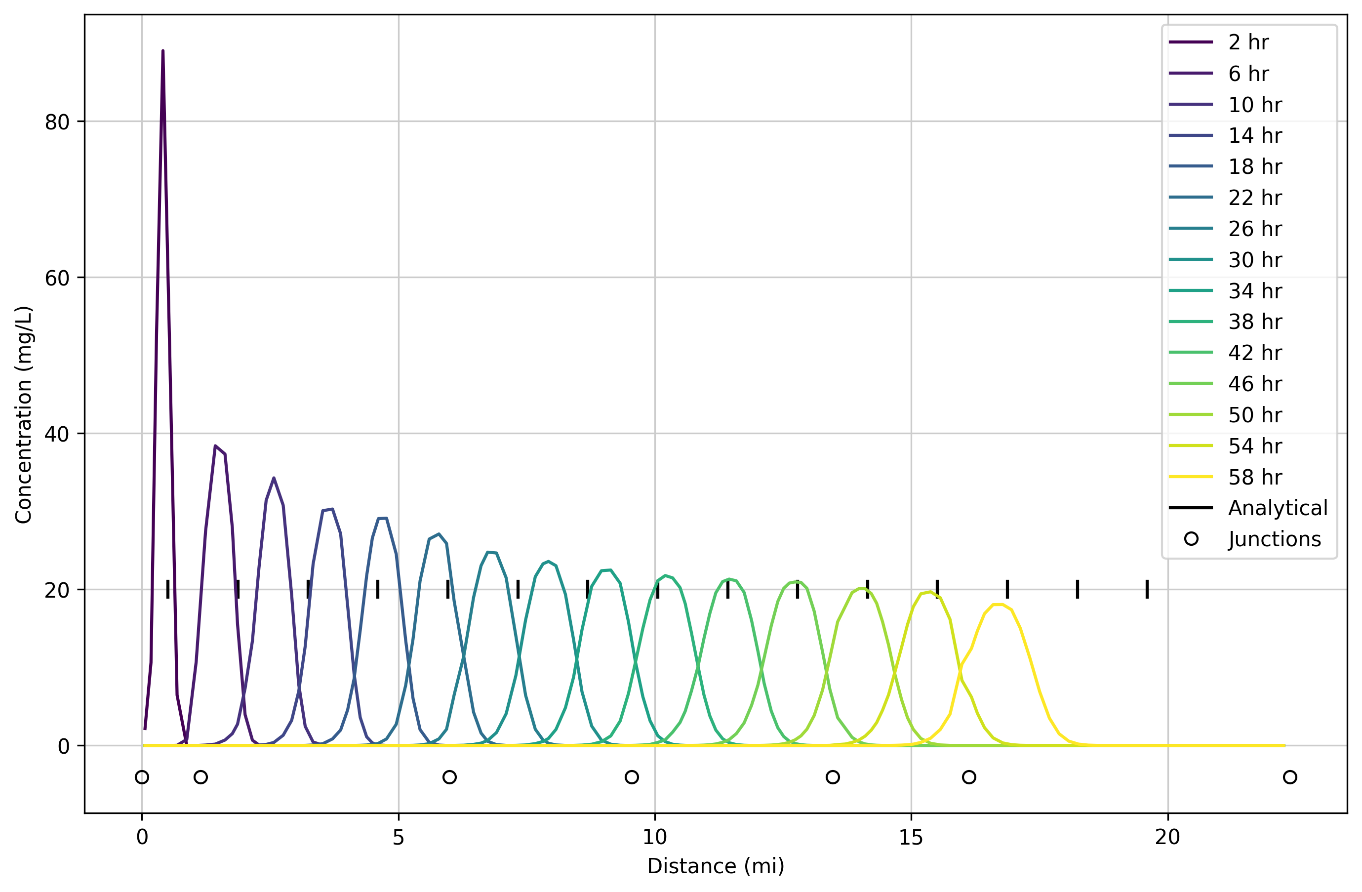
The plot below shows the computed evolution of the initial tracer spike as it is transported downstream through the system. Snapshots of the longitudinal distribution of tracer are shown at four hour intervals following the release. Tick marks along the 20 mg/L line show where the translated analytical solution would be, traveling at an exact speed of 0.5 ft/s. Open circles below the 0 mg/L concentration line show the locations of junctions in ResSim.
The modeled results were obtained using a first order upwind transport method. The method is diffusive, and peak concentrations decrease significantly as the pulse moves downstream. The travel time of the peaks align well with the analytical solution.
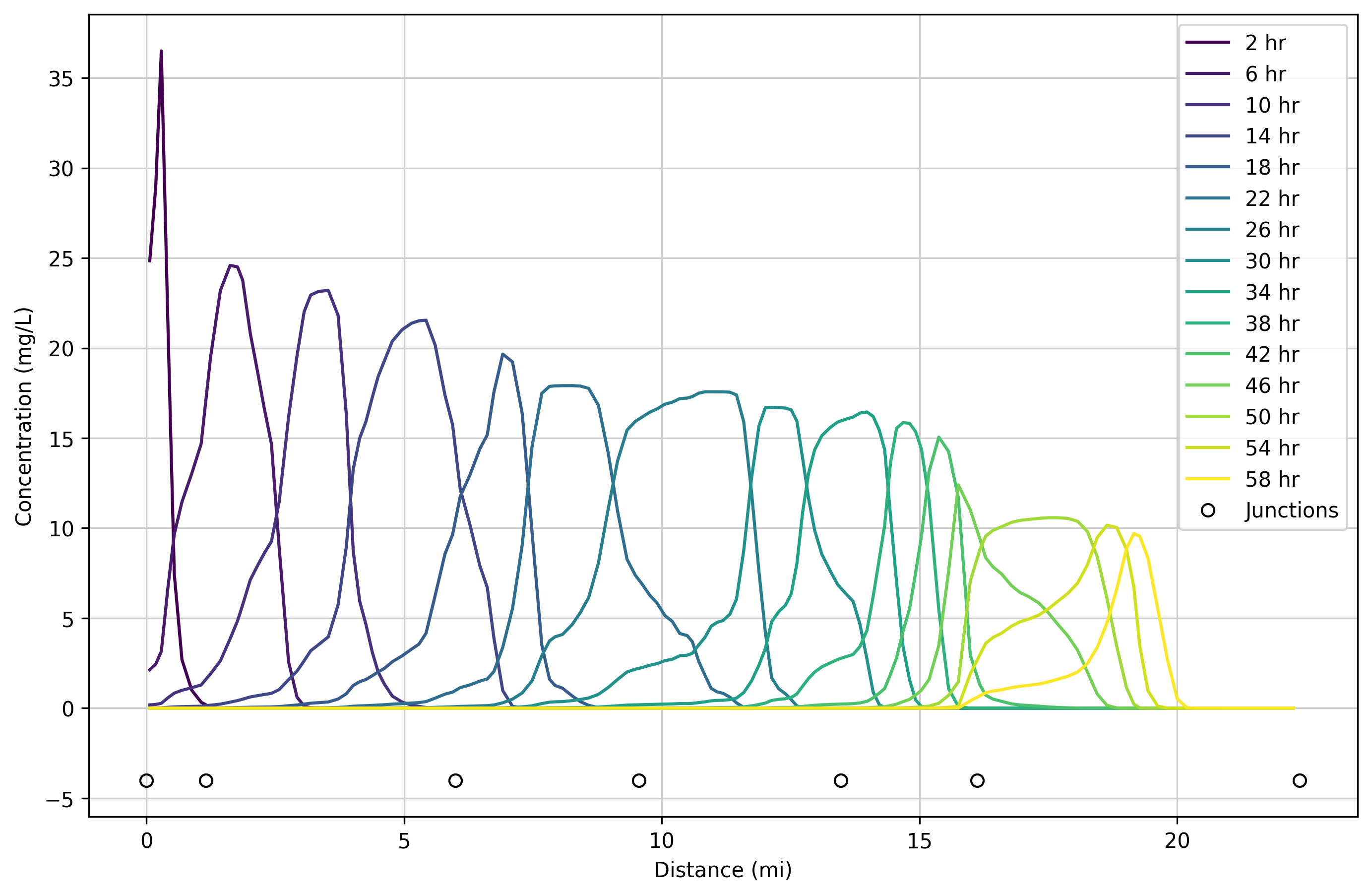
Second order transport
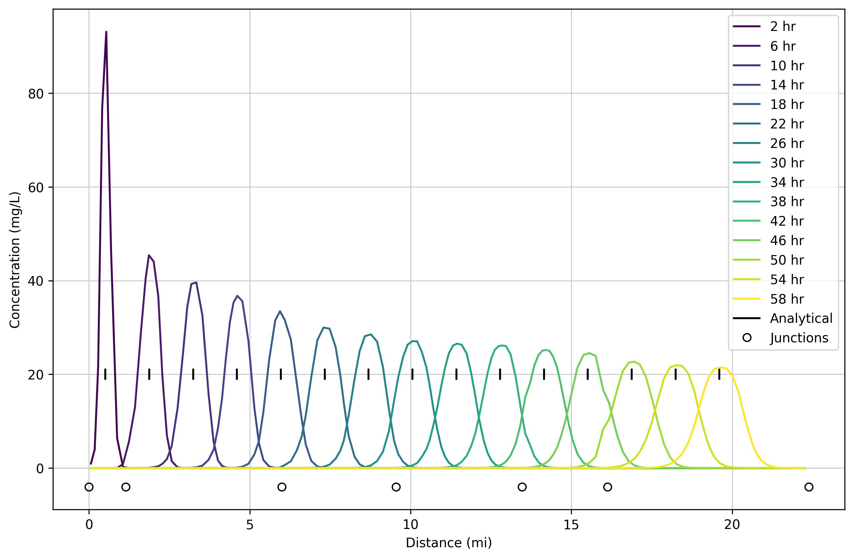
Results using the second order, flux limited transport method (shown below) are significantly less diffusive than the first order method. Travel times remain accurate.
Mass Conservation
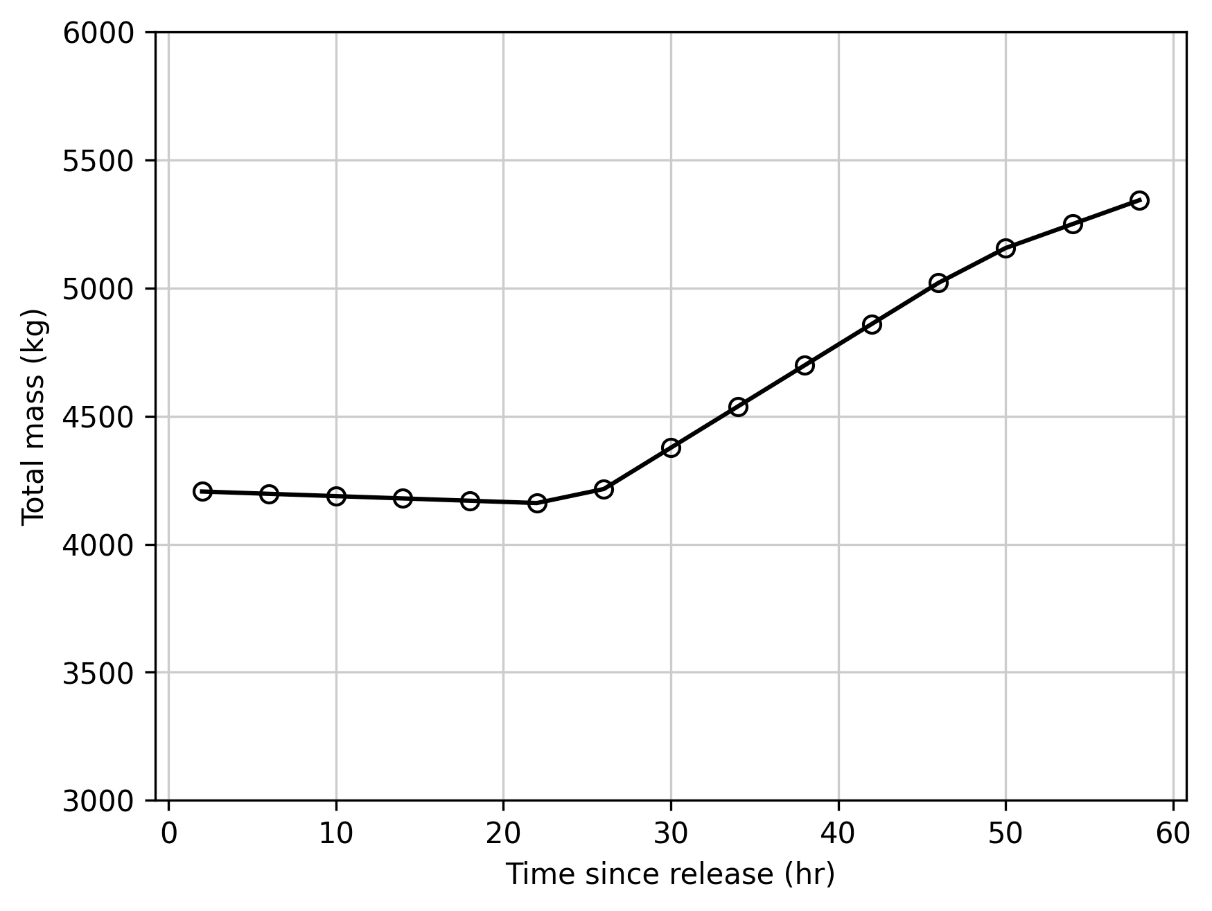
In the above tests, null routing was the applied to all of the reaches and the computational option "Preserve concentration" was selected. (See last section of HEC-ResSim Hydrologic Computations for a description.) A plot of the total mass in the system is shown below, highlighting the lack of mass conservation. After the first day of the simulation, the increasing flows in the system correspond to greater cell volumes and greater average depths. The "Preserve concentration" options adds volume to the cells while maintaining the same concentrations, and leads to an increase is total mass.
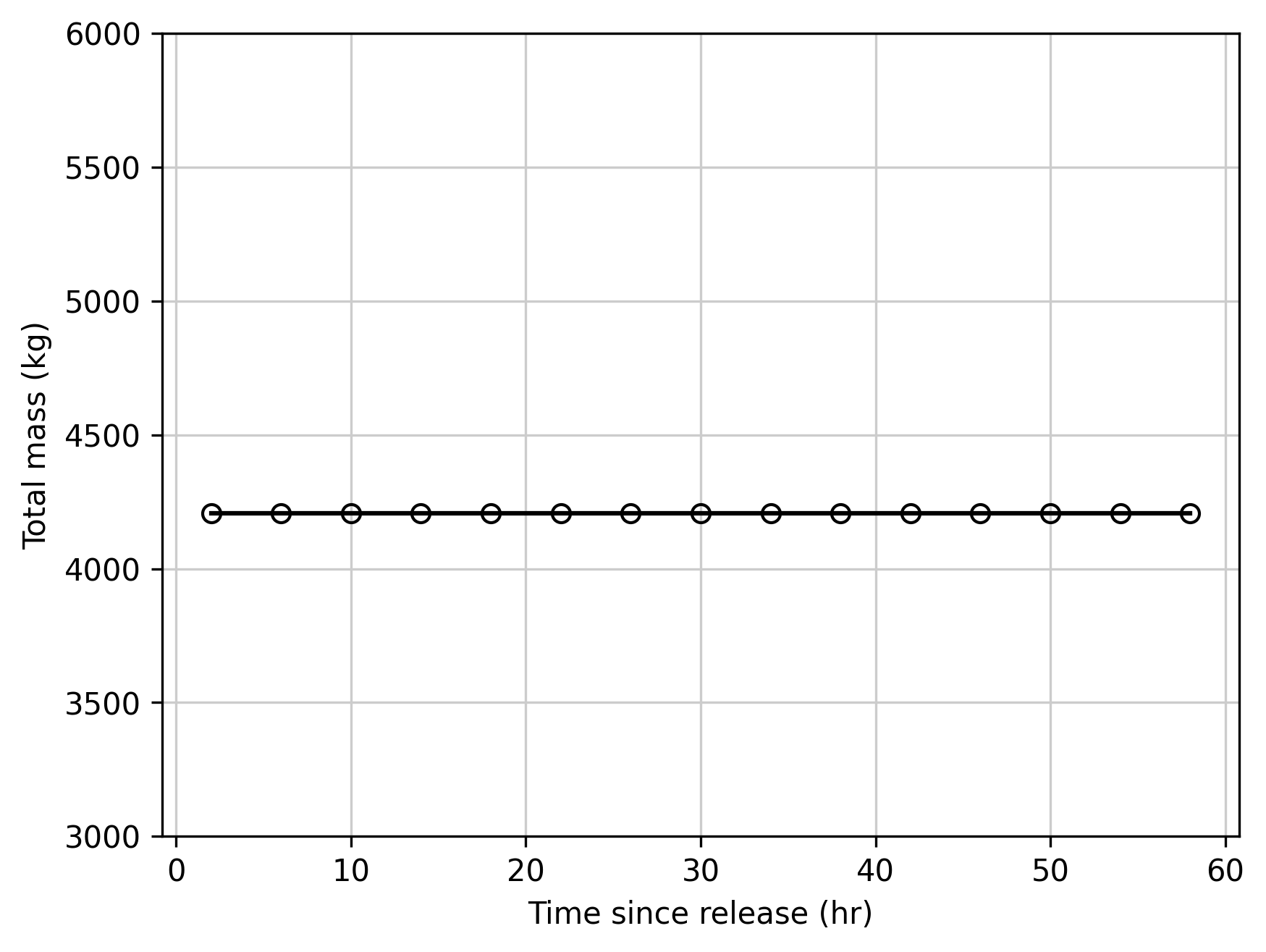
When the "Conserve Mass" computational option is selected, the simulation rigorously applies the finite volume method, and total mass in the system remains constant as the tracer pulse travels downstream.
As discussed in HEC-ResSim Hydrologic Computations, however, this leads to constant cell volumes throughout the simulation. Those cell volumes are set at the start of the simulation (at the start of the "lookback" period in ResSim). With significantly lower flows after the tracer is released, the large cell volumes create longer residence times, and slower effective travel times. The plot below highlights the travel time discrepancy of this method compared to the analytical solution.
Advanced Hydrologic Routing Methods
As mentioned in HEC-ResSim Hydrologic Computations, there are options for more advanced hydrologic routing methods in ResSim which are more conducive to volume conservation over the short time intervals needed for the finite volume transport method. One such method is the Modified-Puls method. This method requires significantly more information than the more simple routing methods, however. In particular, a table of volumes (storages) within each reach segment at a variety of flow rates must be entered. This information can be derived using the HEC-RAS software from a set of steady flow runs. A tutorial for how to create these tables was developed for the HEC-Hydrologic Modeling System (HEC-HMS) documentation and can be found here.
Unfortunately, setting up an analytical test case with constant velocities using this method requires modifications to each of the 243 cross-sections in the RAS model, and was not performed. Instead, the existing RAS cross-sections and steady flow simulations were used to derive storage-discharge tables, and an unsteady simulation was performed in HEC-ResSim using the original, unmodified RAS steady flow table (in order to be consistent with the Mod-Puls storage-discharge tables). The model-computed transport of the tracer pulse is shown below. The shape of the plume warps as it travels through cross-sections with higher or lower velocities, leading to non-symmetric tracer profiles. The pulse moves close to the average low-flow travel speed of 0.5 ft/s, and the total mass is conserved.

Full System Transport Test
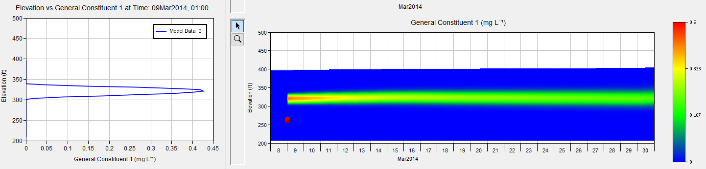
A final test was performed using the full lower American River system, including Lake Folsom and Lake Natoma. The same tracer pulse used for the American River simulations was prescribed at a single upstream boundary inflow to Lake Folsom: a spike of 100 mg/L tracer concentration for one hour at the start of March 9th. Two additional inflows enter the lake, and were not given the tracer spike. At the time of the release, the reservoir is thermally stratified, as shown in the figure below.
The plot below, and the ones following it, were taken from the HEC-ResSim Water Quality Contour Plot results visualization functionality. Information for how to display these plots in ResSim is given in the Water Quality User's Manual. The color contour plot shows the variation of the water quality variable (in this case, water temperature) through time (x-axis) and vertically (y-axis). A red dot on the plot (which may be dragged anywhere through the contour plot by the user) is used to select the time used to extract and plot a one-dimensional vertical profile in the plot window on the left. In the set of plots below, March 9th at 1:00am (just after the tracer release) is selected.
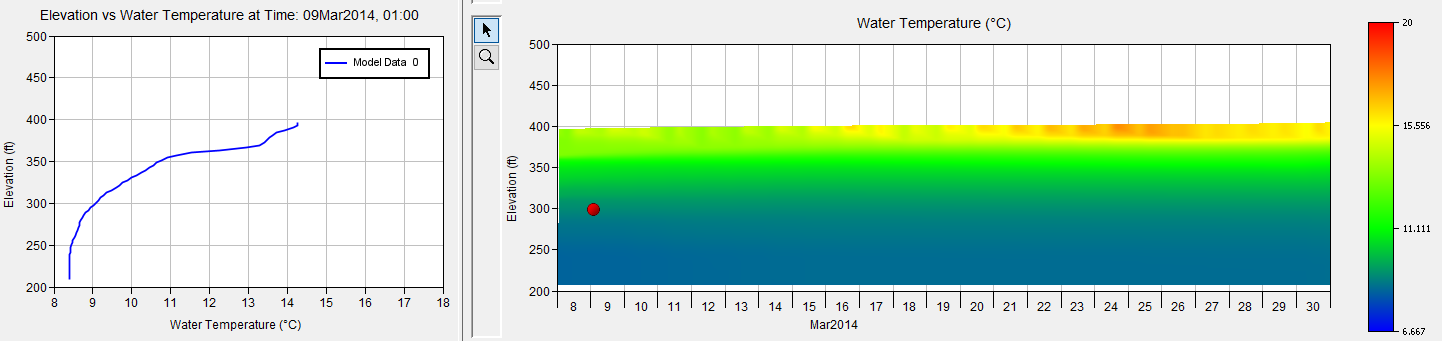
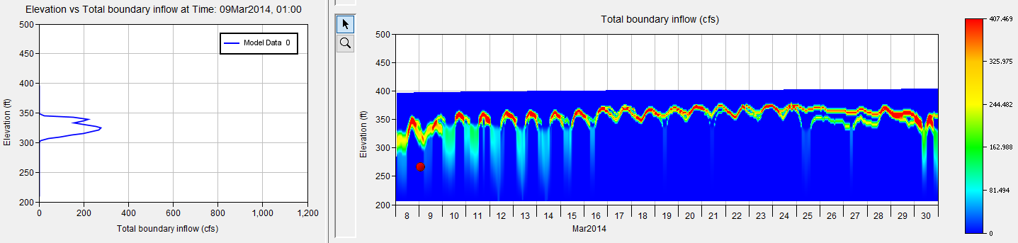
The inflow with the tracer pulse has a temperature at the start of March 9th of 9.8 °C. This leads to an insertion point in the reservoir around 325 ft in elevation. A second major inflow to the lake has a slightly warmer temperature, leading to the bimodal inflow distribution.
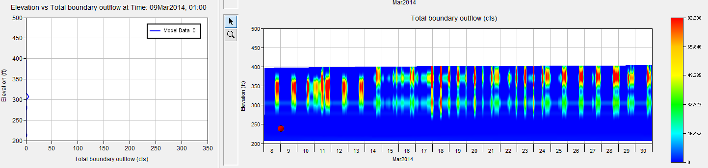
Outflow at the time of the inflow pulse is very small (and includes only reservoir leakage). Peak flows for hydropower generation occur starting in the early evening that day.
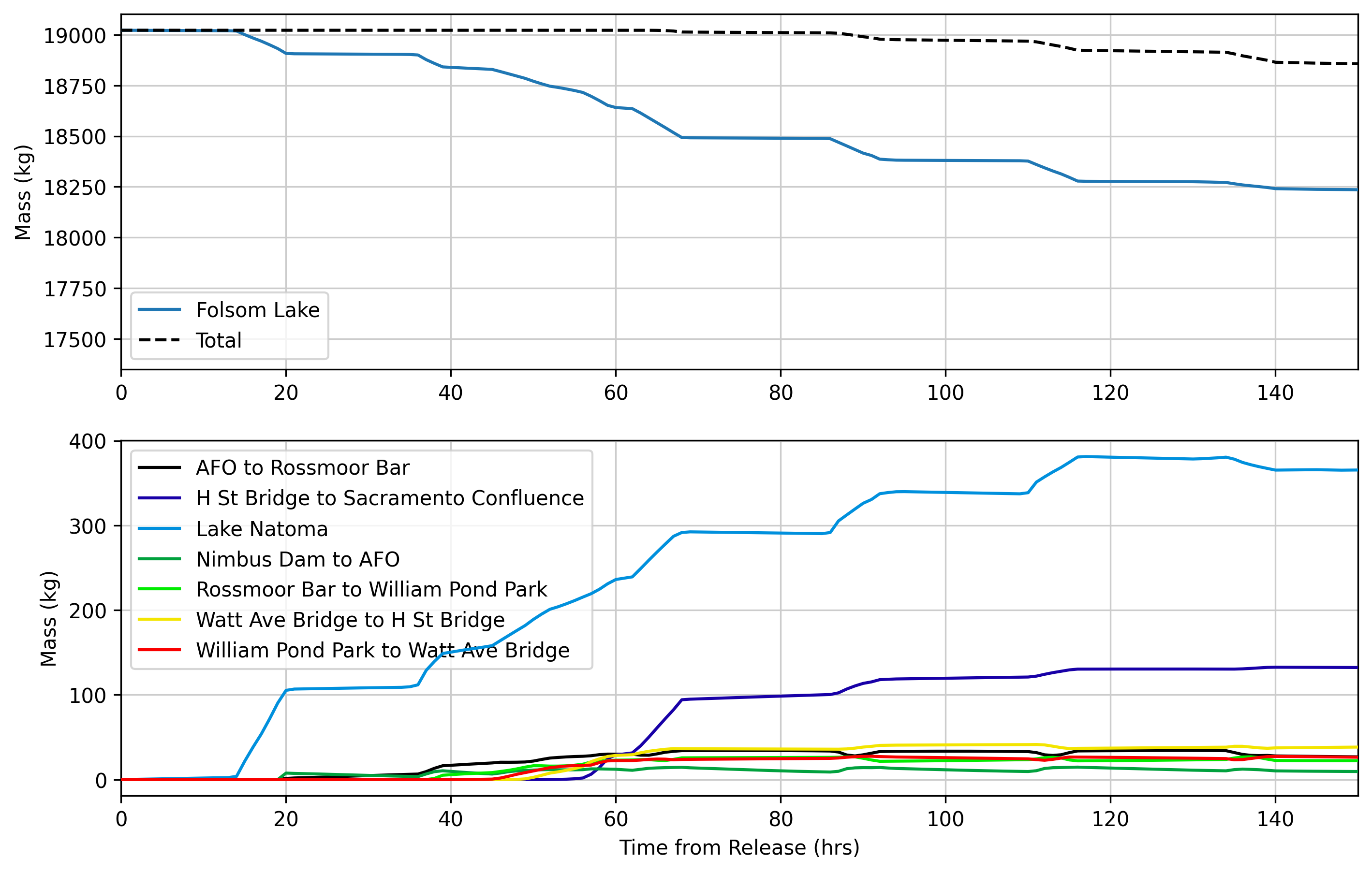
A plot of the total mass in each element of the system is shown below. Folsom and the global total mass are shown on a separate (top) plot because of the large difference in values between those time series and the other element records. The mass in the system remains constant until approximately 70 hours after the tracer release, when the transported tracer begins to reach the boundary at the downstream end of the American River. This demonstrates that a ResSim water quality simulation with multiple element types, inflows, diversions, and complex routing is mass conservative.