Download PDF
Download page Generating a Flow Forecast for International Locations.
Generating a Flow Forecast for International Locations
Software Version
HEC-HMS version 4.11 was used to create this example. You can open the example project with HEC-HMS v4.11 or a newer version.

Introduction
This tutorial is comprised of three major components:
- Delineate a new basin model for an international location starting with terrain data,
- Parameterize the basin model,
- Run an Automated Forecast over the basin model.
If you have already initialized a basin model and are only interested in computing the Automated Forecast, jump to Compute the Automated Forecast.
Study Area
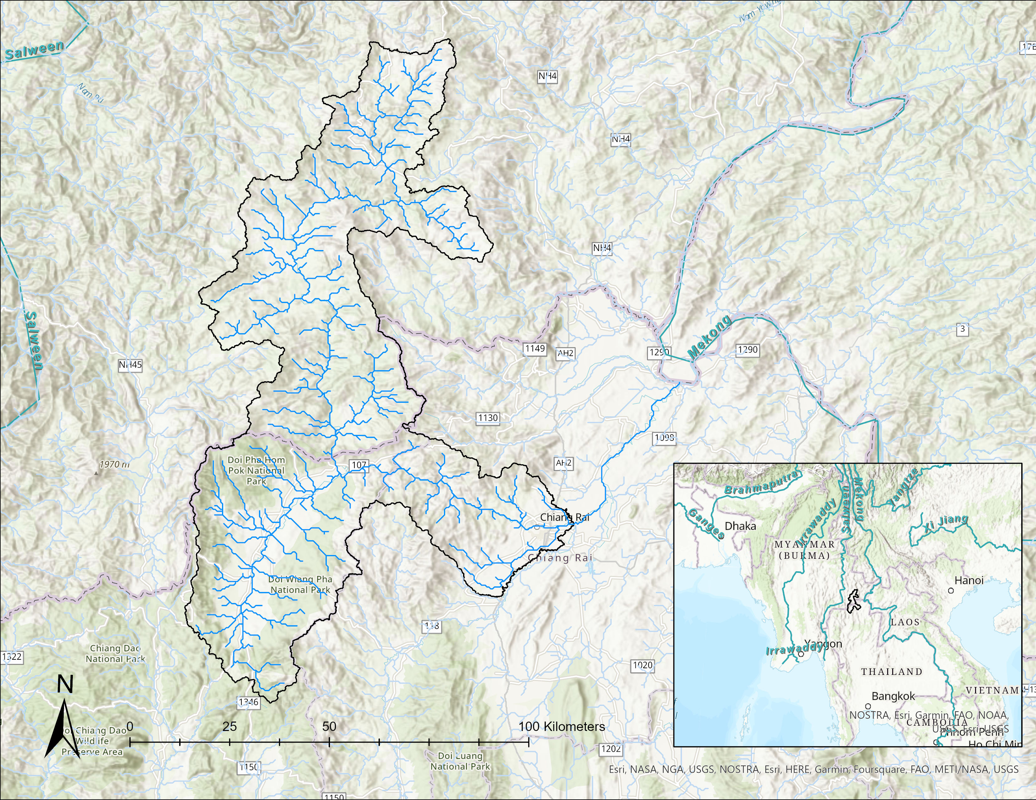
The Automated Forecast feature in HEC-HMS can be used to rapidly generate a flow forecast anywhere on earth. In this example we will develop a flow forecast for the Kok River near Chiang Rai, Thailand. The Kok River originates in Myanmar before flowing into the Chiang Rai province of Thailand and the city of Chiang Rai. Downstream of Chiang Rai, the Kok River flows through an agricultural low land area before joining the Mekong River.
Prepare Terrain Data
NASA's Shuttle Radar Topography Mission (SRTM) data is a global digital elevation model (DEM) dataset and can be used to generate terrain data for HEC-HMS, for any location in the world. In this tutorial the terrain data has already been prepared for you (the terrain data is available at the top of this tutorial). For more information on preparing terrain data for HEC-HMS, see the following tutorials:
Create a New Project
- Open HEC-HMS.
- From the File menu, select New.
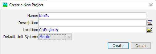
- In the Create a New Project Dialog, name the project KokRv and set the default unit system to Metric.
- Click Create to create the project.
Add Terrain Data
- From the Components menu, select Create Component | Terrain Data.
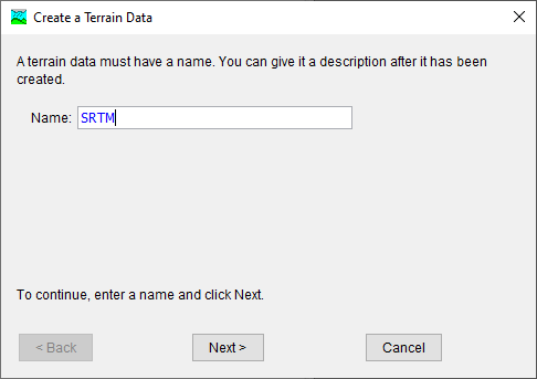
- In the Create a Terrain Data dialog, name the terrain SRTM. Select Next.
- In the Create a Terrain Dialog, set the path to the srtm.tif file. Set the vertical units to Meters. Select Next.
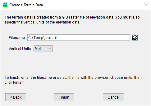
- Click Finish. The Terrain Data has now been created.
The path to terrain data specified above is located external to the project directory. Upon creation of the Terrain Data in HEC-HMS, a copy of the file will be created internal to the project directory.
Create a Basin Model
- From the Components menu, select Create Component | Basin Model.
- In the Create a New Basin Model dialog, name the basin model KokRv.
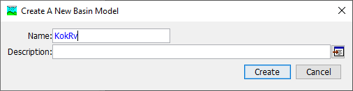
- Click Create. The Basin Model has now been created.
Link Terrain Data to the Basin Model
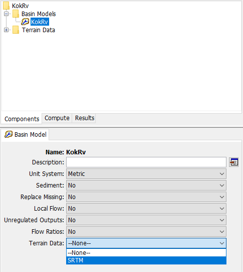
- In the Watershed Explorer, select the KokRv basin model.
- In the Component Editor, set the Terrain Data to SRTM.
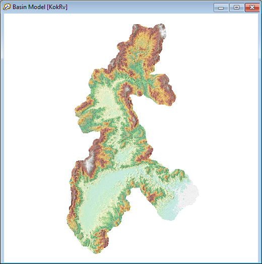
- Click the program Save button. You will be prompted to set the basin model coordinate system. In the Basin Model Coordinate System dialog, select Skip to adopt the coordinate system of the terrain data. The terrain data is in the UTM zone 48 North projection.
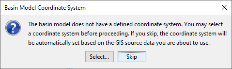
- The terrain data has now been linked to the basin model.
Process the Terrain Data
- From the GIS menu, run the Preprocess Sinks command. This will fill in all local minima in the raster.
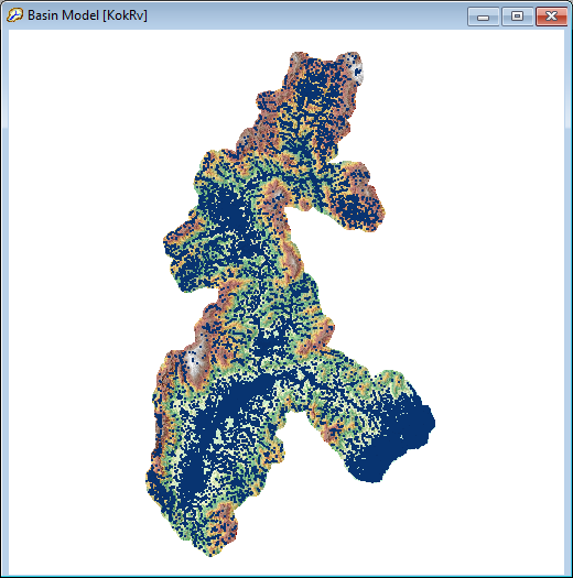
- From the GIS menu, run the Preprocess Drainage command. This will create flow direction and flow accumulation rasters that will be used in subsequent delineation steps.
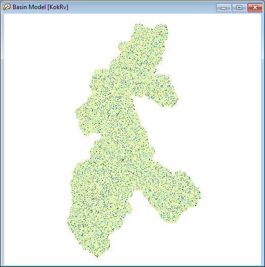
- From the GIS menu, run the Identify Streams command. Set the area to define streams to 400 KM2. This will create an identified stream raster.
Delineate the Basin
- From the GIS menu, select Breakpoint Manager.
- From the Break Points Manager, select Import.
- In the Break Points Importer dialog, specify the path to the breakpoints shapefile (the breakpoint shapefile is available at the top of this tutorial). Select the Snap breakpoints to identified streams option.
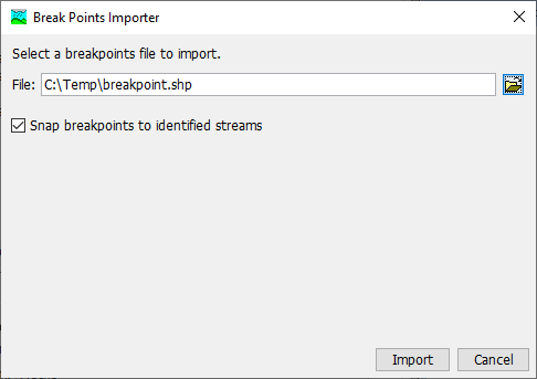
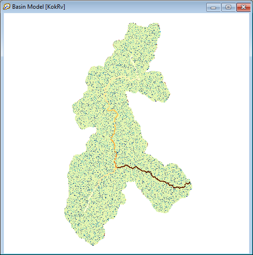
- Select Import. The break point has now been imported and snapped to the nearest identified stream.
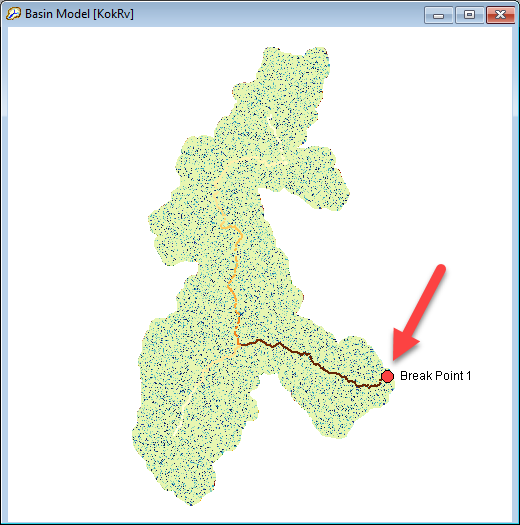
- From the GIS menu, run the Delineate Elements command.
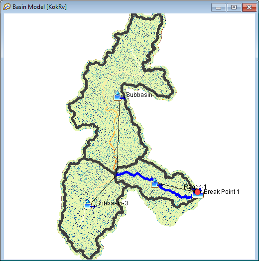
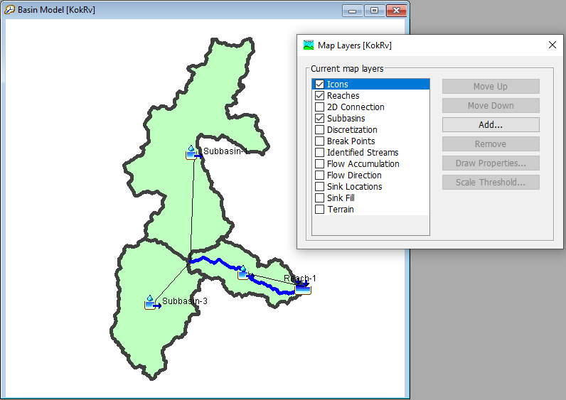
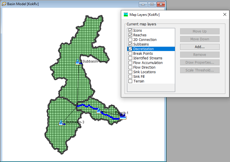
Once delineation is complete you can turn off terrain and terrain-derived map layers. From the View menu, select Map Layers. In the Map Layers dialog, toggle on or off map layers.
Parameterize the Basin Elements
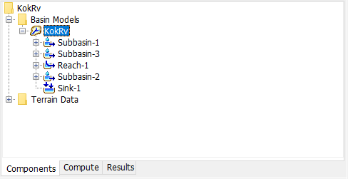
Select the KokRv basin model node in the Watershed Explorer:
Discretization
- With the KokRv basin model node selected, from the Parameters menu, select Discretization | Change Method.
- Select Structured.
- Click Change to set all subbasins to use the Structured discretization method.
- With the KokRv basin model node selected, from the Parameters menu, select Discretization | Structured.
Set Structured discretization parameters according to the table below:
Subbasin Projection Cell Size (meters) Subbasin-1 UTM 48 N 2000 Subbasin-2 UTM 48 N 2000 Subbaisn-3 UTM 48 N 2000 - Click Apply, then Close to commit the edits.
- From the GIS menu, select Compute | Grid Cells to compute grid cell geometries.
Once grid cells are computed, you can visualize this discretization by enabling the Discretization map layer:
Canopy
- With the KokRv basin model node selected, from the Parameters menu, select Canopy | Change Method.
- Select Simple Canopy.
- Click Change to set all subbasins to use the Simple canopy method.
- With the KokRv basin model node selected, from the Parameters menu, select Canopy | Simple Canopy.
Set Simple canopy parameters according to the table below:
Subbasin Initial Storage (%) Max Storage (MM) Crop Coefficient Evapotranspiration Uptake Method Subbasin-1 0 5 1.0 Wet and Dry Periods Simple Subbasin-2 0 5 1.0 Wet and Dry Periods Simple Subbaisn-3 0 5 1.0 Wet and Dry Periods Simple - Click Apply, then Close to save the edits.
Loss
- With the KokRv basin model node selected, from the Parameters menu, select Loss | Change Method.
- Select Deficit and Constant.
- Click Change to set all subbasins to use the Deficit & Constant loss method.
- With the KokRv basin model node selected, from the Parameters menu, select Loss | Deficit and Constant.
Set Deficit and Constant loss parameters according to the table below:
Subbasin Initial Deficit (MM) Maximum Storage (MM) Constant Rate (MM/HR) Impervious (%) Subbasin-1
5 100 2 0.0 Subbasin-2 5 100 2 0.0 Subbasin-3 5 100 2 0.0 - Click Apply, then Close to save the edits.
Transform
- With the KokRv basin model node selected, from the Parameters menu, select Transform | Change Method.
- Select ModClark.
- Click Change to set all subbasins to use the ModClark transform method.
- With the KokRv basin model node selected, from the Parameters menu, select Transform | ModClark.
Set ModClark transform parameters according to the table below:
Subbasin Time of Concentration (HR) Storage Coefficient (HR) Subbasin-1
16 16 Subbasin-2 8 8 Subbasin-3 16 16 - Click Apply, then Close to save the edits.
Baseflow
- With the KokRv basin model node selected, from the Parameters menu, select Baseflow | Change Method.
- Select Linear Reservoir.
- Click Change to set all subbasins to use the Linear Reservoir baseflow method.
- With the KokRv basin model node selected, from the Parameters menu, select Baseflow | Linear Reservoir.
Set Linear Reservoir baseflow parameters according to the table below:
Subbasin Number of Layer Initial Type GW 1 Initial (M3/S /KM2) GW 1 Fraction GW 1 Coefficient (HR) GW 1 Reservoirs GW 2 Initial (M3/S /KM2) GW 2 Fraction GW 2 Coefficient (HR) GW 2 Reservoirs Subbasin-1
2 Discharge Per Area 0.01 0.25
16
2
0.01 0.25
48
4
Subbasin-2 2 Discharge Per Area 0.01 0.25 8
2
0.01 0.25 24
4
Subbasin-3 2 Discharge Per Area 0.01 0.25 16 2 0.01 0.25 48 4 - Click Apply, then Close to save the edits.
Routing
- With the KokRv basin model node selected, from the Parameters menu, select Routing | Change Method.
- Select Lag.
- Click Change to set all reaches to use the Lag routing method.
- With the KokRv basin model node selected, from the Parameters menu, select Routing | Lag.
Set Lag routing parameters according to the table below:
Subbasin Initial Type Lag Time (MIN) Reach-1
Discharge = Inflow 90
- Click Apply, then Close to save the edits.
This model has been parameterized for illustration purposes only. A production forecasting model would be calibrated to events that are of similar magnitude to expected forecasting flow rates.
Compute the Automated Forecast
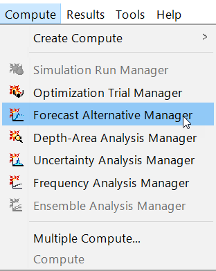
- From the Compute menu, select Forecast Alternative Manager.
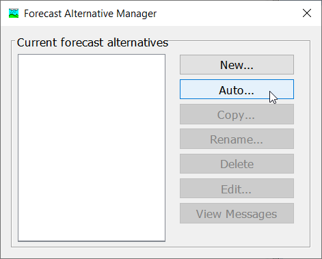
- In the Forecast Alternative Manager, select Auto.
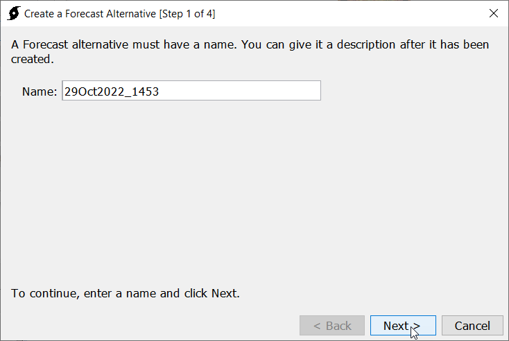
- On Step 1 of the Create a Forecast Alternative wizard, use the default name which corresponds to the current date/time. Click Next.
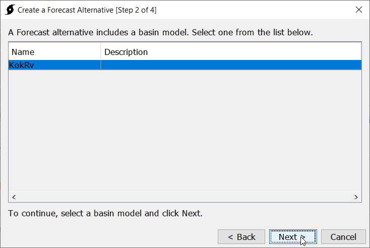
- On Step 2 of the Create a Forecast Alternative wizard, select the KokRv basin model that has been created. Click Next.
On Step 3 of the Create a Forecast Alternative wizard, make no selections. Click Next.
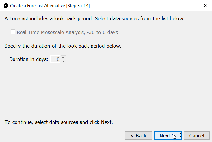

There are not currently any look back period datasets for international locations in the HEC-HMS Automated Forecast. Look back period datasets help establish initial conditions for the forecast simulation. With a good knowledge of soil moisture state at the time of forecast, the look back period can be avoided, but standard practice for USACE is to initialize forecasts with a look back period. If you have a suggestion for near real time data sets of both precipitation and temperature feel free to reach out to the HEC-HMS team.
On Step 4 of the Create a Forecast Alternative wizard, select Global Forecast System (GFS). Click Next.
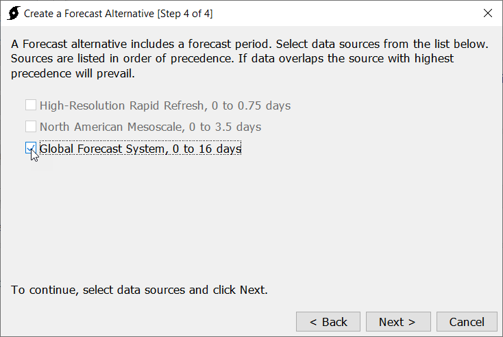
The Global Forecast System (GFS) is a global atmospheric forecast model with forecasted precipitation and temperature for 0 to 16 days from current time.
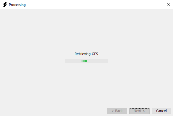
- The Automated Forecast will begin by retrieving forecast data the web:
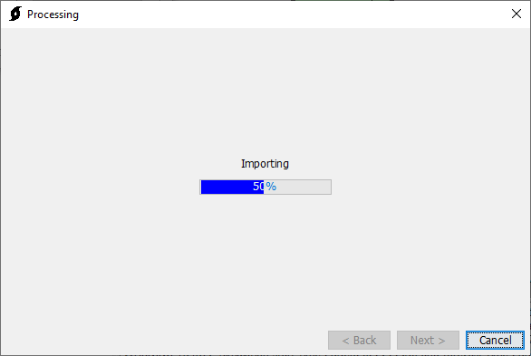
- The Automated Forecast will then import the downloaded data into the HEC-HMS project:
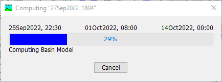
- The Automated Forecast will then run a Forecast Alternative with the imported forecast data:
View Results
You can view results in HEC-HMS by right-clicking on any element in the Basin Map, and selecting View Results.
- Make sure the most recently computed Forecast Alternative is selected in the compute toolbar.
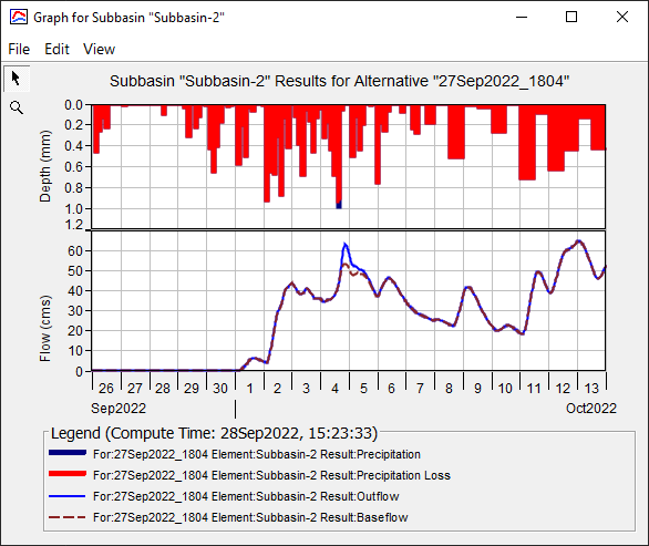
- In the Basin Map, right-click on the Subbasin-2 element, then select View Results | Graph.
- A graph of the computed precipitation and runoff is displayed for Subbasin-2.
Conclusion
In this tutorial we:
- Delineated a new basin model for an international location starting with terrain data,
- Parameterized the basin model,
- Ran an Automated Forecast over the basin model.
The results from the Forecast Alternative can help inform us of an impending flood in the city of Chiang Rai, or help us forecast inflows to the irrigation dam near Wiang Chai, downstream of Chiang Rai.