Download PDF
Download page Creating and Calibrating the Oct2010 Simulation.
Creating and Calibrating the Oct2010 Simulation
Return to Creating Boundary Conditions for the Magat River Basin Model
Last Modified: 2023-06-20 15:31:07.993
Software Version
HEC-HMS version 4.11 was used to create this tutorial. You will need to use HEC-HMS version 4.11, or newer, to open the project files.
Project Files
If you are continuing from Creating Boundary Conditions for the Magat River Basin Model you can continue to use your current project files. Otherwise download the initial project files here:
Create an Oct2010 Control Specification
Control specifications define the temporal extent and resolution of the simulation.
- In HEC-HMS, select Components | Create Component | Control Specification.
- Name the Control Specification Oct2010.
- In the Watershed Explorer, select the Oct2010 Control Specification node.

- In the Component Editor, set Start Date: 18Oct2010, Start Time: 0000, End Date: 25Oct2010, and End Time: 2400. Set the time interval to 1 Hour.

- Click the program Save button.
Create an Oct2010 Simulation
- In HEC-HMS, select Compute | Create Compute | Simulation Run.
- Name the Simulation Oct2010. Select the MagatRv basin model, the Oct2010 meteorologic model, and the Oct2010 control specification.
- Run the Oct2010 Simulation.
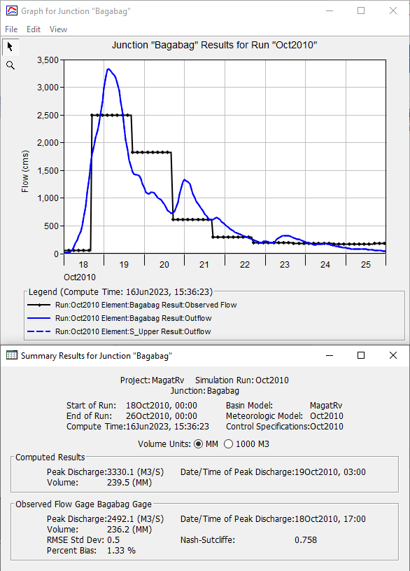
- Inspect the results. View the result graph
 and summary table
  for the Bagabag junction, as shown below.
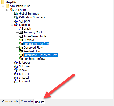
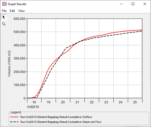
- Also, plot the Cumulative Outflow and Observed Cumulative Outflow time series for the Bagabag junction. To plot these time series, first navigate to the Results tab, expand the Simulation Runs node, the Oct2010 node, the Bagabag node, and select the Cumulative Outflow and Observed Cumulative Outflow time series, as shown below.

Use the Shift and Ctrl keys to select multiple time series at once.
- Then, click the result graph button to plot these time series in a new window, as shown below.

- Leave the plots and summary table open so you can see results change as you modify parameters.
- Notice that the computed results match the observed results fairly well. However, the computed results slightly overpredict the cumulative outflow on the rising limb of hydrograph for this event on October 18 and 19, 2010. Thus, modifications to the initial loss, transform, baseflow, and channel routing parameters should be made to improve the agreement between the computed and observed results.
The computed results are available at the computational time step (i.e., 1 hour). However, the observed results are only available as daily averages. Thus, direct comparisons between the computed peak flow rate and observed peak flow rate are not easily made.
Calibrate the Basin Model
For more in-depth coverage of model calibration for events, see Calibrating and Validating a Single Event Model.
- Adjust model model parameters to achieve an acceptable level of agreement between computed and observed flow. Use the result graph, summary table, and Cumulative Outflow vs Observed Cumulative Outflow time series plot to gauge the effectiveness of your parameter modifications.
Canopy
| Subbasin | Initial Storage (%) | Max Storage (MM) | Crop Coefficient | Evapotranspiration | Uptake Method |
|---|---|---|---|---|---|
| S_Upper | 0 | 5 | 1.0 | Wet and Dry Periods | Simple |
| S_Lower | 0 | 5 | 1.0 | Wet and Dry Periods | Simple |
| S_Local | 0 | 5 | 1.0 | Wet and Dry Periods | Simple |
Loss
| Subbasin | Initial Deficit (MM) | Maximum Storage (MM) | Constant Rate (MM/HR) | Impervious (%) |
|---|---|---|---|---|
S_Upper | 10 | 100 | 5 | 0.0 |
| S_Lower | 10 | 100 | 5 | 0.0 |
| S_Local | 10 | 100 | 5 | 0.0 |
Transform
| Subbasin | Time of Concentration (HR) | Storage Coefficient (HR) |
|---|---|---|
S_Upper | 10 | 5 |
| S_Lower | 10 | 5 |
| S_Local | 5 | 2.5 |
Baseflow
| Subbasin | Number of Layer | Initial Type | GW 1 Initial (M3/S /KM2) | GW 1 Fraction | GW 1 Coefficient (HR) | GW 1 Reservoirs |
|---|---|---|---|---|---|---|
S_Upper | 1 | Discharge Per Area | 0.05 | 1 | 10 | 1 |
| S_Lower | 1 | Discharge Per Area | 0.05 | 1 | 10 | 1 |
| S_Local | 1 | Discharge Per Area | 0.05 | 1 | 10 | 1 |
Routing
| Subbasin | Initial Type | Lag Time (MIN) |
|---|---|---|
R_Upper | Discharge = Inflow | 180 |
R_Local | Discharge = Inflow | 60 |
The image below shows a calibrated hydrograph at the Bagabag junction:

In this model observed data is only available for one of three subbains in our model. One strategy for modeling ungaged basins is to model nearby gaged basins with similar characteristics and apply calibrated parameters to ungaged basins. In this example we calibrated the S_Upper subbasin and let that calibration inform our parameterizations of the S_Lower and S_Local subbasins. A more complete analysis of ungaged basins would include calibration of more nearby gaged basins with multiple events. Regressions can be made between calibrated parameters and basin characteristics.
Summary
A simulation run was created and computed. The basin model was calibrated to a single historical event.
In this example, the basin model was calibrated to a single historical event. A production forecasting model should be calibrated to multiple events of similar magnitude and antecedent conditions in order to be accurate.
Continue to Running an Automated Forecast for the Magat River Basin
