Download PDF
Download page W5 - Calibrating an HEC-HMS Model.
W5 - Calibrating an HEC-HMS Model
Overview
In this workshop you will calibrate an HEC-HMS model to a modeling application. Initial parameter estimates will be estimated using GIS information and the model will be calibrated through trial and error. HEC-HMS version 4.9 was used to created this workshop. You will need to use HEC-HMS version 4.9, or newer, to open the project files.
Download the Initial project files here - start_Calibration_Workshop.zip
Estimate Initial Parameter Values
A Note on Parameter Estimation
The values presented in this workshop are meant as initial estimates. This is the same for all sources of similar data including Engineer Manual 1110-2-1417 Flood-Runoff Analysis and the HEC-HMS Technical Reference Manual. Regardless of the source, these initial estimates must be calibrated and validated.
Deficit and Constant Loss
GIS information and techniques presented within the W1 - Applying the Deficit and Constant Loss Method workshop were used to estimate Deficit and Constant loss parameters for each subbasin within the study area.
| Subbasin | Initial Deficit (in) | Maximum Deficit (in) | Constant Rate (in/hr) |
|---|---|---|---|
| MF_American_Rv_S30 | 0.5 | 4.3 | 0.19 |
| Duncan_Ck_S10 | 0.5 | 4.6 | 0.17 |
| MF_American_Rv_S20 | 0.5 | 3.5 | 0.16 |
| MF_American_Rv_S10 | 0.5 | 1.6 | 0.08 |
Clark/ModClark Unit Hydrograph
The regression equations and techniques presented within the W2 - Applying the Clark/ModClark Unit Hydrograph Method workshop were used to estimate ModClark unit hydrograph parameters for each subbasin within the study area.
| Subbasin | L (mi) | DA (sq mi) | S1085 (ft/ft) | LSqrtDAS | RR | Tc (hr) | R (hr) |
|---|---|---|---|---|---|---|---|
| MF_American_Rv_S30 | 17.7 | 47.2 | 0.01937 | 875.3 | 0.04044 | 3.2 | 2.9 |
| Duncan_Ck_S10 | 15.8 | 23.6 | 0.03582 | 404.5 | 0.04919 | 2.9 | 2.0 |
| MF_American_Rv_S20 | 9.1 | 11.2 | 0.03815 | 156.2 | 0.06198 | 2.6 | 1.4 |
| MF_American_Rv_S10 | 5.2 | 7.0 | 0.0389 | 69.3 | 0.11796 | 2.6 | 1.2 |
Linear Reservoir Baseflow
The information and techniques presented within the W3 - Applying the Linear Reservoir Baseflow Method workshop were used to estimate Linear Reservoir baseflow parameters for each subbasin within the study area.
| Subbasin | # Layers | GW 1 | GW 2 | ||||||
|---|---|---|---|---|---|---|---|---|---|
| Initial (cfs/sq mi) | Fraction | Coefficient (hr) | # Reservoirs | Initial (cfs/sq mi) | Fraction | Coefficient (hr) | # Reservoirs | ||
| MF_American_Rv_S30 | 2 | 0 | 0.5 | 8.6 | 1 | 0 | 0.5 | 28.7 | 1 |
| Duncan_Ck_S10 | 2 | 0 | 0.5 | 6.1 | 1 | 0 | 0.5 | 20.2 | 1 |
| MF_American_Rv_S20 | 2 | 0 | 0.5 | 4.2 | 1 | 0 | 0.5 | 13.9 | 1 |
| MF_American_Rv_S10 | 2 | 0 | 0.5 | 3.7 | 1 | 0 | 0.5 | 12.4 | 1 |
Muskingum-Cunge Channel Routing
GIS information and techniques presented within the W4 - Applying the Muskingum-Cunge Routing Method workshop were used to estimate Muskingum-Cunge channel routing parameters for each routing reach within the study area.
| Reach | Length (ft) | Slope (ft/ft) | Manning's n | Space-Time Method | Index Celerity (ft/s) | Shape | Bottom Width (ft) | Side Slope (ft/ft) |
|---|---|---|---|---|---|---|---|---|
| MF_American_Rv_R20 | 43824 | 0.04 | 0.035 | Auto DX Auto DT | 5 | Trapezoid | 27 | 0.56 |
| MF_American_Rv_R10 | 23707 | 0.037 | 0.035 | Auto DX Auto DT | 5 | Trapezoid | 70 | 0.5 |
Enter Parameter Values and Compute a Simulation
- Open the Calibration_Workshop project and then open the Dec_1996_Jan_1997 Basin Model.
- Select Parameters | Loss | Deficit and Constant to open the Deficit and Constant Global Editor, as shown in the following figure.

- Enter the initial Deficit and Constant loss parameters for each subbasin that were shown above.
- Select Parameters | Transform | ModClark to open the ModClark Global Editor.
- Enter the initial ModClark transform parameters for each subbasin that were shown above.
- Select Parameters | Baseflow | Linear Reservoir to open the Linear Reservoir Global Editor.
- Enter the initial Linear Reservoir baseflow parameters for each subbasin that were shown above.
- Select Parameters | Routing | Muskingum-Cunge to open the Muskingum-Cunge Global Editor.
- Enter the initial Muskingum-Cunge routing parameters for each routing reach that were shown above.
- Select the Dec_1996_Jan_1997 simulation run from the Compute toolbar,
 .
. - Press the Compute All Elements button,
 , to run the simulation.
Calibrate the Model Upstream of French Meadows Reservoir
We will start adjusting our parameters to better match the observed inflow to French Meadows Reservoir. The loss, transform, and baseflow parameters for the subbasin upstream of French Meadows Reservoir have already been calibrated within the previous workshops. However, you will repeat these steps again to gain familiarity with calibrating an HEC-HMS model. The tutorial below will walk you through one way of systematically calibrating your model to match the observed hydrograph. We will work through adjusting initial baseflow, then move onto losses, then adjusting your unit hydrograph parameters, then lastly your baseflow parameters. Other hydrologists and engineers may have their own calibration techniques. Keep in mind that calibration is an iterative process! Just because one parameter looks good after your first adjustment doesn't mean you won't need to go back and refine the parameter value again; however, calibration should be more than just adjusting parameters to best match a curve. It is also important to have a good understanding of the watershed hydrology and know what are the reasonable ranges for model parameters. If your watershed consists of mainly sandy, well draining soils, it wouldn't make much sense to set your loss rates to 0 inches per hour just so you can match your hydrograph volume. Have a reason to why you are making your adjustment. Parameter values should make sense to the watershed and the types of events you are modeling. This will allow you to have confidence in your model results and defend your modeling results when you're able to explain the why behind the values. When you start needing to adjust your model beyond reasonable limits, this may suggest issues with your model boundary conditions, your model set up, or something more fundamental about your basin that isn't being captured.
Modify the MF_American_Rv_S30 Subbasin Element
- Begin by viewing the result graph,
 , and summary table,
  , for the MF_American_Rv_S30 subbasin element.
 - Modify the initial baseflow parameters to approximately match the initial discharge at the start of the simulation.
- Once you have adequately matched the initial discharge, continue by modifying the loss parameters to approximately match the initiation of runoff.
- Next, modify the loss parameters to approximately match the observed runoff volume.
- Now, move onto modifying the unit hydrograph parameters to approximately match the rising limb of the observed data.
- Once the rising limb of the observed data has been adequately matched, modify the unit hydrograph parameters to approximately match the receding limb of the observed data.
- Next, modify the baseflow parameters to match the receding limb of the observed data.
- Finally, iteratively modify loss, transform, and baseflow parameters to achieve an adequate fit to the observed data.
Review Results
At this point, we've made initial adjustments to the computed hydrograph for the MF_American_Rv_S30 subbasin element. You may have noticed that adjustments for one parameter could affect another part of the hydrograph you did not intend to change. For example, while increasing the GW 1 & 2 coefficients for baseflow, the hydrograph peak was reduced. Unless there is a compelling reason, avoid making drastic adjustments to one parameter to compensate for an adjustment to another. Continue to keep in mind reasonable parameter ranges as you make your adjustments and that the parameters you are selecting make sense for your basin.
If you haven't already noticed, the summary table provides statistical metrics that can be used to assist in calibration. For instance, a useful metric commonly used is the Nash-Sutcliffe Efficiency (NSE), which measures the predictive skill of a hydrologic model. A value of "1" means the simulated values can perfectly predict the observed where there is no estimation error variance, while a value of "0" means the estimation error variance is equal to the error variance in the observed data. Moriasi, et. al, 2007 developed a performance rating table based on commonly used statistical measures to evaluate model performance.
Performance Rating | NSE | RSR | PBIAS |
|---|---|---|---|
Very Good | 0.65<𝑁𝑆𝐸≤1.00 | 0.00<𝑅𝑆𝑅≤0.60 | 𝑃𝐵𝐼𝐴𝑆< ±15 |
Good | 0.55<𝑁𝑆𝐸≤0.65 | 0.60<𝑅𝑆𝑅≤0.70 | ±15≤𝑃𝐵𝐼𝐴𝑆<±20 |
Satisfactory | 0.40<𝑁𝑆𝐸≤0.55 | 0.70<𝑅𝑆𝑅≤0.80 | ±20≤𝑃𝐵𝐼𝐴𝑆<±30 |
Unsatisfactory | 𝑁𝑆𝐸≤0.40 | 𝑅𝑆𝑅>0.80 | 𝑃𝐵𝐼𝐴𝑆≥±30 |
This can be one of several methods to assess model performance. However, similar to the issue with curve fitting, the modeler should not focus solely on maximizing NSE or another, single metric. The calibration process should also take into account the needs of the project (i.e. concerned with peak flow, volume, or both) and you're understanding of the watershed through research and analysis.
The statistical metrics that are reported within the summary table are computed using the simulation time step (i.e. 15 minutes). The observed data used for calibration is daily average. This causes a conflict and results in poor NSE and RSR statistical metrics that are reported. To compute more appropriate statistical metrics, the computed output should be converted to the same time step as the observed data. Future enhancements within HEC-HMS will aid modelers when these situations are encountered.
Calibrate the Model Downstream of French Meadows Reservoir
Now that the subbasin element upstream of French Meadows Reservoir has been adequately calibrated, the three subbasins and two routing reaches in between French Meadows Reservoir and Interbay Dam need to be calibrated as well.
- Begin by viewing the result graph and summary table for the Interbay_Dam_In junction element.
- Change the Linear Reservoir baseflow initial discharge to approximately match the observed data at the start of the simulation.
- Select Parameters | Baseflow | Linear Reservoir to open the Linear Reservoir Global Editor.
- Uniformly modify the initial baseflow parameters for the Duncan_Ck_S10, MF_American_Rv_S20, and MF_American_Rv_S10 subbasin elements, as shown in the following image.

- Click the Compute All Elements button within the Linear Reservoir Global Editor,
 , to run the simulation.
 - Inspect the results for the Interbay_Dam_In junction and repeat as necessary to match the observed data at the start of the simulation.
- Once you have adequately matched the initial discharge, continue by modifying the loss parameters to approximately match the initiation of runoff.
- Select Parameters | Loss | Deficit and Constant to open the Deficit and Constant Global Editor.
- Modify the Initial Deficit parameters for each subbasin to approximately match the initiation of runoff.
- Click the Compute All Elements button within the Deficit and Constant Global Editor to run the simulation.
- Inspect the results for the Interbay_Dam_In junction and repeat as necessary to approximately match the initiation of runoff.
- Continue modifying the loss parameters to approximately match the observed instantaneous peak discharge (13900 cfs).
- Within the Deficit and Constant Global Editor, select the Constant Rate cells for the Duncan_Ck_S10, MF_American_Rv_S20, and MF_American_Rv_S10 subbasin elements, right click, and select Fill, as shown in the following image.

- Select the Multiple by Constant radio button and enter a value of 0.5, as shown in the following figure.
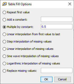
- Click OK to multiply the currently selected values by 0.5.
- Click the Apply button to apply the changes.
- Click the Compute All Elements button within the Deficit and Constant Global Editor to run the simulation.
- Inspect the results for the Interbay_Dam_In junction and repeat as necessary to approximately match the observed peak discharge.
- Within the Deficit and Constant Global Editor, select the Constant Rate cells for the Duncan_Ck_S10, MF_American_Rv_S20, and MF_American_Rv_S10 subbasin elements, right click, and select Fill, as shown in the following image.
- Continue modifying the loss parameters to approximately match the observed runoff volume.
- Use the Deficit and Constant Global Editor to modify parameters.
- Now, move onto modifying the unit hydrograph parameters to approximately match the rising limb of the observed data.
- Use the ModClark Global Editor to modify parameters.
- Once the rising limb of the observed data has been adequately matched, modify the unit hydrograph parameters to approximately match the receding limb of the observed data.
- Use the ModClark Global Editor to modify parameters.
- Next, modify the baseflow parameters to match the receding limb of the observed data.
- Use the Linear Reservoir Global Editor to modify parameters.
- Now, modify the routing parameters for the MF_American_Rv_R20 and MF_American_Rv_R10 reaches to better match the arrival time of the computed hydrograph.
- Also, ensure no oscillations due to the computational time step or parameterization are present.
- Use the Muskingum-Cunge Global Editor to modify parameters.
- Finally, iteratively modify loss, transform, baseflow, and routing reach parameters to achieve an adequate fit to the observed data. Keep track of the differences between observed peak discharge, runoff volume, and overall hydrograph fit.
Different modelers may arrive at different parameter combinations when calibrating. Understanding how different processes and parameters impact the computed results is more important than obtaining a "perfect" fit within this workshop.
Questions
Question 1. How do the results look compared to the simulated results?
The computed inflow to French_Meadows_Reservoir and computed pool elevation match the observed data well, as shown in the following figures.


However, the computed results at the Interbay_Dam_In junction overpredict the runoff volume by approximately 50% while matching the reported instantaneous peak discharge of 13900 cfs, as shown in the following figure.

This overestimation needs to be weighed against the project goals. If producing the correct runoff volume is more important than producing the correct peak discharge, then parameter modification geared towards that goal should be pursued.
Question 2. What physical considerations should be used when calibrating?
Model parameters must make physical sense and be regionally consistent. For instance, using a constant loss rate of 1 in/hr within a single subbasin in order to achieve an adequate fit to the observed data is not appropriate. First off, a constant loss rate that large within this modeling domain is not physically reasonable. Second, using a constant loss rate within one subbasin that is significantly different from nearby subbasins cannot be easily justified. When physically unreasonable parameters are required to achieve an adequate fit, errors in boundary conditions or other model parameters should be investigated.
Question 3. Which parameter(s) had the largest impact when calibrating?
Increasing the constant loss rate parameter by a factor of 3 (i.e. initial value * 3; initial value / 3) resulted in relatively large impacts of approximately 25% to the computed peak flow rate. However, due to the use of the Linear Reservoir baseflow method, losses due to the constant loss rate are returned as baseflow. As such, less drastic changes on the order of 10% to the computed runoff volume are realized with changes to this parameter.
Increasing/decreasing the time of concentration and storage coefficient by a factor of 3 results in an approximate 10% difference in computed peak discharge. Due to the use of the Linear Reservoir baseflow method, unit hydrograph parameter changes do not affect the computed runoff volume.
Making reasonable changes to the initial deficit (i.e. ~0.5 inches to ~1.5 inches) resulted in relatively small impacts on the computed results at the Interbay_Dam_In junction. Runoff volume is decreased when the initial deficit is increased.
Increasing the GW1 and GW2 coefficients by a factor of 5 results in only moderate impacts to the computed hydrograph at the Interbay_Dam_In junction (approximately 2% decrease in computed peak discharge)
Decreasing the GW1 and GW2 partition fractions so that all infiltrated water is lost to a deep aquifer can reduce the computed peak discharge by approximately 15% while reducing the runoff volume by approximately 23%. However, using this parameter combination would require significant physical justification. A more reasonable combination of 0.4/0.4 results in more justifiable results.
Changing the Muskingum-Cunge routing parameters resulted in little to no appreciable differences to peak discharge, volume, and/or hydrograph shape at the Interbay_Dam_In junction.
Question 4. Were meteorologic inputs and/or parameter(s) modified during calibration? Should they be investigated and/or modified during a real study?
This calibration exercise was simplified in order to fit within the allotted time. As such, several parameters were not highlighted for modification. These include precipitation and temperature data sources as well as temperature index snowmelt parameters, amongst others.
Within a real study, additional precipitation and temperature data sources should be investigated to ensure that the boundary conditions are accurate and appropriate for use within model calibration.
Temperature index snowmelt parameters should definitely be modified during model calibration. Observed snow data (e.g. University of Arizona, SNODAS, etc) can be used to compare the computed outputs.
Additional Task: Calibrate to the February 1986 Event
Now that you've calibrated one basin model, use your newfound talents to calibrate another event. It is good practice to calibrate your hydrologic model to more than 1 storm event. Model parameters are not static values that exist without variability. On the contrary, given the heterogeneity that exists within the watershed basin with differing soil types, changes in land use and vegetation as well as differing antecedent soil conditions, model parameters and their associated watershed response are expected to change for different storm events. This is another important reason to understand how your model predictions will be used and to tailor your calibration events to reflect what will be predicted. For example, if you are interested in estimating the 1% annual chance exceedance event, you'll want to look at storm events that produced high flows and not storms that produce average flows.
Another large storm event within the study area occurred in February 1986. During this flood, 13 Californians lost their lives while over 14,000 homes and 1100 businesses were damaged (CNRFC, https://www.cnrfc.noaa.gov/storm_summaries/feb1986storms.php).
- Create a copy of the Dec_1996_Jan_1997 basin model. Name this new basin model Feb_1986.
- Select the GriddedData_1986 meteorologic model, select the Basins tab, and ensure the Feb_1986 basin model is selected.
- Create a new simulation run and name it Feb_1986.
- Select the Feb_1986 basin model, GriddedData_1986 meteorologic model, and Feb_1986 control specifications.
- Make parameter modifications to the Feb_1986 basin model to better recreate the runoff conditions that persisted during this flood event.