Download PDF
Download page Debris Yield Modeling Using Erosion Methods in HEC-HMS.
Debris Yield Modeling Using Erosion Methods in HEC-HMS
Last Modified: 2023-02-23 09:06:49.585
This tutorial demonstrates a process to estimate post fire debris using HEC-HMS.
Software Version
HEC-HMS version 4.11 was used to develop this tutorial.

Introduction
The Hermits Peak Fire began on April 4, 2022 in New Mexico, and burned 74% of the Gallinas Creek Watershed. In this tutorial you will use 5 debris yield methods to calculate the post-wildfire sediment load of each subbasin and determine the bulking factor for the entire Gallinas Creek Watershed.
Basin Model Setup for Post-Fire Sediment Analysis
- Copy one of the post-fire basin models by right clicking on the basin model and selecting Create Copy…
- Remove all the reaches from one of the post-fire basin models created in this tutorial by right clicking on each reach element and selecting Delete.
- For this effort, reaches are removed because of time restraints, limitations in current debris-routing methods, and a lack of data to calibrate the model.
- Note: While HEC-HMS has the capability to route debris yield from subbasins through the reaches and reservoirs, new methods ("Sediment Delivery Ratio" (SDR) transport potential method and "Muskingum" routing method) specific to debris flow routing are being developed for the reach element to improve model accuracy.
- Note: Multiple reaches can be selected by holding down the "Ctrl" key and deleted at once.
- For this effort, reaches are removed because of time restraints, limitations in current debris-routing methods, and a lack of data to calibrate the model.
Filling Out Properties in the Sediment Tab
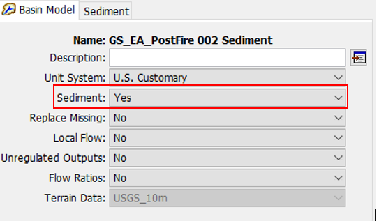
- Set Sediment to "Yes" in the Basin Model tab.
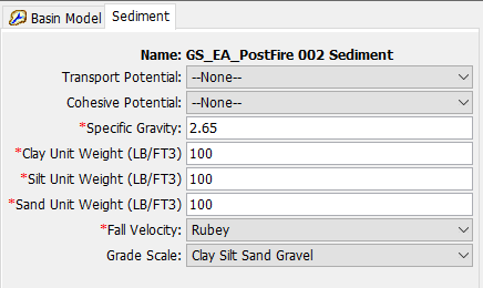
- Set the Specific Gravity to 2.65, which is the default value.
- Set the Unit Weight for all three soil types to 100 lb/ft3.
- Set the Fall Velocity method to "Rubey".
- Note: The fall velocity only applies to reach and reservoir elements, so even though a fall velocity is selected, it will not be used in this simulation.
- Set the Grade Scale to "Clay Silt Sand Gravel".
Selecting a Debris Yield Method for Post-Fire Modeling
- Set the debris yield method by going to Parameters | Erosion, then clicking on the appropriate debris yield method.
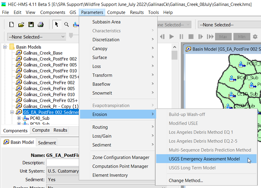
- For this tutorial, five debris yield methods were used to compare the computed sediment yield for each method, but this is not necessary for all modeling efforts.
- The five debris yield methods utilized for this effort were: Los Angeles Debris Method EQ 1, Los Angeles Debris Method EQ 2-5, Multi-Sequence Debris Prediction Method, USGS Emergency Assessment Model, and the USGS Long Term Model.
- The five methods used are described in detail here:
- Fill out the input parameters for each debris yield method. The 5 debris yield methods used in the model are described in detail below.
LA Debris Method Equation 1
This method can be applied to subbasins that are less than 3 mi2.
- Flow Rate Threshold1: Set the flow rate threshold to 1.0594 cfs, which is the minimum direct runoff flow rate that will generate debris yield.
- Adjustment/Transposition Factor (A-T Factor)2: set the A-T factor to 1.
- Relief Ratio: The relief ratio can be found in the HEC-HMS Subbasin Characteristics by clicking on Parameters | Characteristics | Subbasin.
- Convert the relief ratio into units of ft/mi by multiplying the value by 5,280 ft/mi.
- Fire Factor Type: Set to "User-Specified."
- Fire Factor: The Fire Factor is given a value of 3 if the entire subbasin is unburned and a value of 6.5 if the entire subbasin is burned. If there is a mix of unburned and burned areas within the subbasin, the equation below should be used.
Fire Factor=(3*Area Unburned+6.5*Area Burned)/Total Area - Exponent3: Set the exponent to 1.
- Gradation Curve: Use the curve that was developed in this tutorial - Gradation Curve Development Procedure.
LA Debris Method Equation 2-5
This method can be applied to subbasins that are 0.1 to 200 mi2.
- Flow Rate Threshold1: Set the flow rate threshold to 1.0594 cfs, which is the default value in HEC-HMS.
- Adjustment/transposition factor (A-T Factor) 2: set the A-T factor to 1.
- Relief Ratio: The relief ratio can be found in the HEC-HMS Subbasin Characteristics by clicking on Parameters | Characteristics | Subbasin.
- Convert the relief ratio into units of ft/mi by multiplying the value by 5,280 ft/mi.
- Fire Factor Type: Set to "User-Specified."
- Fire Factor: The Fire Factor is given a value of 3 if the entire subbasin is unburned and a value of 6 if the entire subbasin is burned. If there is a mix of unburned and burned areas within the subbasin, the equation below should be used.
- Note: The Fire Factor was selected based on Figure 3 in the USACE's "Los Angeles District Method for Prediction of Debris Yield" report and is dependent on the subbasin area and the years since the fire.
Fire Factor=(3*Area Unburned+6.0*Area Burned)/Total Area
- Note: The Fire Factor was selected based on Figure 3 in the USACE's "Los Angeles District Method for Prediction of Debris Yield" report and is dependent on the subbasin area and the years since the fire.
- Exponent3: Set the exponent to 1.
- Gradation Curve: Use the curve that was developed in this tutorial - Gradation Curve Development Procedure.
Multi-Sequence Debris Prediction Method (MSDPM)
This method can be applied to subbasins that are 0.1 to 3.0 mi2.
- Adjustment/transposition factor (A-T Factor) 2: set the A-T factor to 1.
- Relief Ratio: The relief ratio can be found in the HEC-HMS Subbasin Characteristics by clicking on Parameters | Characteristics | Subbasin.
- Convert the relief ratio into units of ft/mi by multiplying the value by 5,280 ft/mi.
- Maximum 1-HR Rainfall Intensity: Set to 0.001.
- Total Minimum Rainfall Amount: Set to 0.001.
- Fire Factor Method: Set to "User-Specified"
- Fire Factor: The Fire Factor is given a value of 3 if the entire subbasin is unburned and a value of 6.5 if the entire subbasin is burned. If there is a mix of unburned and burned areas within the subbasin, the equation below should be used.
Fire Factor=(3*Area Unburned+6.5*Area Burned)/Total Area - Flow Rate Threshold1: Set the flow rate threshold to 1.0594 cfs, which is the default value in HEC-HMS.
- Exponent3: Set the exponent to 1.
- Gradation Curve: Use the curve that was developed in this tutorial - Gradation Curve Development Procedure.
USGS Emergency Assessment Debris Model
This method can be applied to subbasins that are 0.004 to 12.7 mi2.
- Relief: Set the relief equal to the Basin Relief, which is found in the HEC-HMS Subbasin Characteristics by clicking on Parameters | Characteristics | Subbasin.
- Burn Area: Set the burn area to the total area within the watershed that was impacted by the fire.
- Use results from this tutorial to calculate the burned area - Watershed Burn Severity Calculation Procedure.
- Flow Rate Threshold1: Set the flow rate threshold to 1.0594 cfs, which is the default value in HEC-HMS.
- Exponent3: Set the exponent to 1.
- Gradation Curve: Use the curve that was developed in this tutorial - Gradation Curve Development Procedure.
USGS Long-Term Debris Model
This method can be applied to subbasins that are 0.004 to 12.7 mi2.
- Relief: Set the relief equal to the Basin Relief, which is found in the HEC-HMS Subbasin Characteristics by clicking on Parameters | Characteristics | Subbasin.
- Burn Date: Set the date to the end of the fire.
- Burn Area: Set the burn area to the total area within the watershed that was burned at moderate and high severity.
- Use results from this tutorial to calculate the burned area - Watershed Burn Severity Calculation Procedure.
- Flow Rate Threshold1: Set the flow rate threshold to 1.0594 cfs, which is the default value in HEC-HMS.
- Exponent3: Set the exponent to 1.
- Gradation Curve: Use the curve that was developed in this tutorial - Gradation Curve Development Procedure.
Notes from Superscripts:
- The flow rate threshold sets the minimum direct runoff flow for which debris yield will be calculated.
- The A-T factor accounts for debris yield volume differences between the San Gabriel Mountains (the location of the data used to develop the original linear regression equations for the LA Debris Methods), and the modeled reach. If it is known that debris yield volumes will be less than or greater than the measured volumes for the San Gabriel mountains, an A-T factor can be set, which will multiply the volume that is computed from the linear regression equations.
- The exponent changes the shape of the debris yield curve relative to the hydrograph. By setting the exponent to 1, the shape of the debris hydrograph will mirror the water hydrograph.
Creating Unique Post-Fire Basin Models for Various Frequencies
If unique basin models were created for each frequency in the pre-fire calibration, separate basin models for each frequency also need to be generated for debris yield simulations.
- Copy the newly created basin model that has a sediment method and no reaches.
- Change the loss and transform parameters to the post-fire CN and lag times.
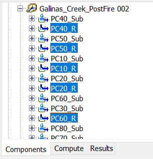
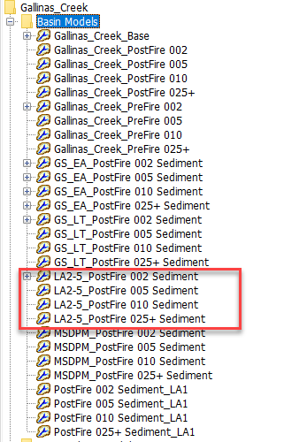
- Repeat for all frequencies. The figure below shows the basin models configure for the Gallinas Creek HEC-HMS model. Notice there is a separate set of basin models for each debris method and there are four basin models that cover the frequency events.
Simulation Runs for Post-Fire Debris Yield
- Create new meteorological models for each frequency.
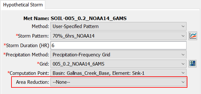
- Copy the hypothetical storm meteorological models that were previously developed and change the Area Reduction to "None."
- Note: The area reduction is removed so that the computed results provide more conservative estimates for the sediment load and the estimated bulking factor.
- Note: The area reduction is removed so that the computed results provide more conservative estimates for the sediment load and the estimated bulking factor.
- Create a control specification.
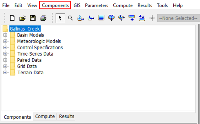
- Create a control specification by clicking Components | Control Specifications Manager.
- Create a control specification by clicking Components | Control Specifications Manager.
- Next, click on the New… button to create a new control specification.
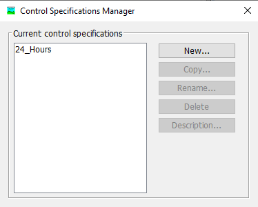
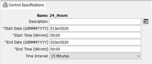
- Enter a Start Date and an End Date in the Control Specifications.
- The duration set in the control specifications needs to be long enough to capture the entire hydrograph of every subbasin within the watershed.
- For the Gallinas Creek model, 24 hours is sufficient.
- Note: The start date does not matter unless you are using the USGS Long-Term Debris Model or Pak & Lee Fire Factor Method because these methods require a burn date.
- The duration set in the control specifications needs to be long enough to capture the entire hydrograph of every subbasin within the watershed.
- Copy the hypothetical storm meteorological models that were previously developed and change the Area Reduction to "None."
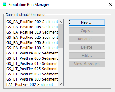
- Create a simulation run for each debris yield method and frequency.
- Create a simulation run by clicking Compute | Simulation Run Manager.
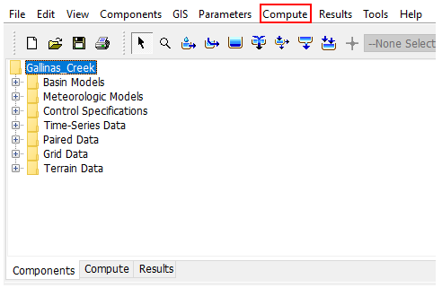
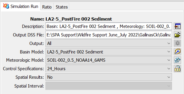
- Next, click on the New… button to create a new simulation run and fill out the name of the simulation run. Next, select the basin model, meteorological model, and control specification when prompted to do so. Then click Finish.
- Make sure the basin model and meteorological model represent the same return period.
- Make sure the basin model and meteorological model represent the same return period.
- Below is an example of the inputs for an event with a return period of 2 years (50% annual exceedance probability) and uses the LA Debris Method Equation 2-5 as the erosion method.
- Create a simulation run by clicking Compute | Simulation Run Manager.
- Now that the simulation run has been setup, click the compute button.

Results
- Go to the Results tab and click on the Global Summary.
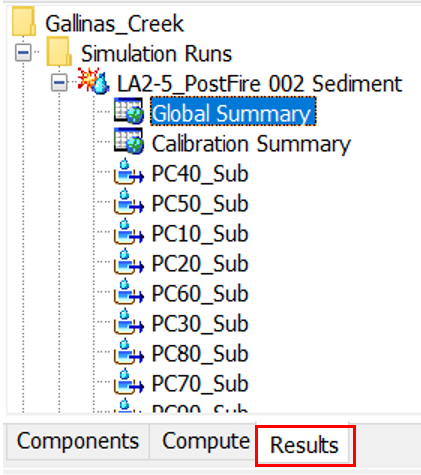
- The Global Summary has the results for the Sediment Volume of each subbasin. Calculate the sum of the sediment volume for all the subbasins.
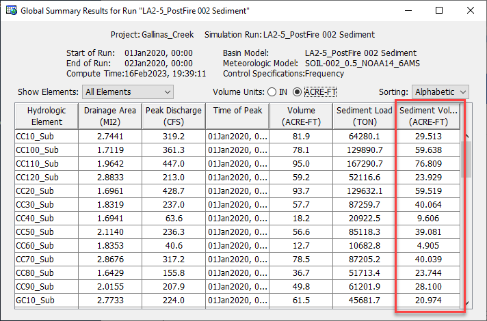
- Calculate the sum of the water volume and sediment volume for all the subbasins.
- Calculate the bulking factor using the equation below:
BF=(Vs+Vw) / Vw
Where BF is the bulking factor, Vs is the volume of sediment/debris, and Vw is the volume of water. The total water volume, total sediment volume, and bulking factor for an event with a return period of 2 years (50% annual exceedance probability) and uses the LA Debris Method Equation 2-5 can be seen in the table below.
Total Water Volume (acre-ft)
Total Sediment Volume (acre-ft)
Bulking Factor
2213.3
1083.6
1.49
Repeat this process for all frequencies and erosion methods.
References
Gatwood, E., Pedersen J., and Casey, K. 2000. Debris Method: Los Angeles District Method for Prediction of Debris Yield. U.S. Army Corps of Engineers, Los Angeles District, Los Angeles, CA. Gatwood_2000_Los+Angeles+District+Debris+Method.pdf