In this tutorial, you will create:

• Grid Data components that represent point precipitation-frequency in space, and
• Time series of spatially-distributed rainfall grids.

This tutorial can be completed independently, beginning with a fresh version of the HEC-HMS project available on the Shared Component Data Overview page, or continuing from the Creating Paired Data tutorial.

Software Version

HEC-HMS version 4.12 beta 3 was used to create this example. You can open the example project with HEC-HMS 4.12 or a newer version.

Project Files

Download initial project files provided on the Shared Component Data Overview page

Step 1. Begin by opening the project in HEC-HMS 4.12 Beta 3 or later.

You will see that this project has a basin model already created for you. If you are continuing on from other Shared Component Data tutorials, you may also see time series data or paired data in your project.

Creating a Grid Data Component (General Overview)

In HEC-HMS, a Grid Data shared component is a container for multiple types of data that can be represented as a regular lattice, or grid. To create a new Grid Data, choose the Components menu in the menu toolbar, select Create Component | Grid Data.

 Components | Create Component | Grid Data.

A window will prompt you for a name, description and data type. Note that there are two general types of grids in this list: those ending in Gridsets, and those ending in Grids. Gridsets, in general, represent a time-series of grids, and are typically hydrometeorological boundary conditions such as precipitation and temperature grids in time. Grids are static and generally represent spatially distributed hydrologic parameters such as moisture deficit or percolation rate.

The following tutorial will demonstrate the difference between these two types of data using a static grid (a precipitation-frequency grid) and a gridset (a time series of precipitation grids.)

Importing a Precipitation-Frequency Grid

Precipitation-frequency grids are used within the Hypothetical Storm precipitation method in the Meteorology Model. They represent the rainfall depth associated with a specific duration of rainfall, and average exceedance probability. For example a precipitation-frequency grid might represent the depth of rain associated with the 24-hour accumulation, and an annual exceedance probability of 1%. NOAA Atlas 14 provides precipitation-frequency estimates for most of the United States, and the resulting point-precipitation frequency estimates are provided as spatial data. They are commonly available from the NOAA Precipitation Frequency Data Server as ASCII-format raster files.

For this workshop, a copy of the 24-hour 1% annual exceedance probability precipitation-frequency grid for the Ohio River Basin project area from NOAA PFDS has been provided in the project data folder:

NOTE that *.prj file is required to provide spatial reference for gridded data.

Step 2. Begin by creating a new Precipitation-Frequency grid by using the Components menu (see the beginning of this tutorial.) When the creation window comes up, select the Precipitation-Frequency Grid data type (near the bottom of the list.)

Step 3. Then, name the grid data 24hr 100yr. Providing a description is optional but generally good practice. After providing a name and description, select Create and a new grid data component will be created.

Step 4. You will find the new grid data in the Watershed Explorer under a new folder called Grid Data. Underneath that folder in the tree will be another folder called Precipitation-Frequency Grids. HEC-HMS organizes all of its grids by data type, and all data types are distinct grids from one another. Underneath the Precipitation-Frequency Grids folder will be the grid data you just created. Click on that grid data to select it and open its properties in the Component Editor:

Step 5. The settings for the grid are used to link the Shared Component Data to data on disk. For most grid types, the data is stored only in Single Record HEC-DSS files. However, to make precipitation-frequency grids easier to work with, the ASCII grid option is available for these data. For the Data Source, select ASCII. You will see the other options change in response.

Step 6. For the Filename, use the file browser option (the folder icon) to navigate to the project folder, and then to the data folder inside of that. In that folder you should only see one file called orb100yr24ha.asc. Select this file and select Open.

Step 7. The Filename text box will be populated. You will also need to specify the Units and Unit Scale Factor. NOAA Atlas 14 data are stored in 1000ths of inches, so select "in" for Units, and 1000 for Unit Scale Factor. A unit scale factor is typically used to store floating point data as integers, with the scale factor selected in order to preserve the desired level of precision. Your options should look like the following:

Step 8. Finally, save your project by using the Save button in the toolbar or by pressing Ctrl+S.

Importing Gridsets

Importing precipitation gridsets from the original data involves a two step-process. HEC-HMS uses HEC-DSS to store all grid data and gridsets. First, data from any other source (such as GRIB or NetCDF) must be imported into an HEC-DSS file. Then, an HEC-HMS grid can be linked to the HEC-DSS file.

Importing GRIB-Format Grid Data to DSS

GRIB is a common format for storing meteorological data. One common source of precipitation data is the multi-radar multi-sensor (MRMS) dataset, which is commonly available in GRIB format. 24 hours of hourly MRMS precipitation are provided with the tutorial project in the data folder. The MRMS data contain a far larger domain than the project area, so clipping out the area of interest is helpful. Doing so requires a shapefile of the project domain, which can be created by HEC-HMS. The result of this first process is to create an HEC-DSS file containing the precipitation gridset of interest, for the project domain. It will still need to be linked to a Grid Data inside of HEC-HMS.

Export Project Elements as Shapefile

Step 9. Export the subbasin shapefile for the project by first selecting the Sep2018 basin model in the Watershed Explorer, and then choosing from the GIS menu Export Layers.

Step 10. You will then see a wizard appear. In the first step, accept the default options (to export subbasin elements) by selecting Next  in the bottom-center. On the second step of the wizard you will see an option to set the destination file. Click on the folder icon to the right of the Filename (*.shp) text field to open the file browser. Navigate to the data folder inside your HEC-HMS project. Once inside that folder, specify the filename as punx_subbasin and select Save.

Step 11. This will return you to the second step of the wizard. Complete the wizard by selecting Finish in the bottom-center. This will create the necessary boundary shapefile in the data folder.

Use the Data Importer

Step 12. Next, open the File menu and select File | Import  | Gridded Data | Importer.

Step 13. You will see the Gridded Data Import Wizard open. Click on the folder icon to browse to the data directory of your HEC-HMS project.

Step 14. Inside of the data directory is a folder called QPE. Open that folder, and you should see 24 MRMS QPE files, one for each hour of 01 September 2018. Press Ctrl+A to select all files, and then press Open.

Step 15. The list of files inside the import wizard will be populated with the 24 GRIB files you just selected. Press Next to go to the next step.

Step 16. You should see the variable selection panes. Select variable called GaugeCorrQPE01H_altitude_above_msl in the left pane, and press the ">" button to import that variable. Then, press Next to go to the next step.

Step 17. In this step you will specify the geometric options for the import. The first field is for the clipping datasource. We will use the shapefile we exported in an earlier step. Click on the folder icon to the right of the Clipping datasource text field to browse to the punx_subbasin.shp file in the data folder, created earlier. Next, specify a target wkt (well-known text representation of coordinate reference system) by selecting the globe icon to the right of the text field of the Target wkt text field. This will open a list of pre-defined projections. The default option of SHG is good, so select Ok in this window. The target wkt text field will be populated with the SHG wkt. Next, specify the target cell size by clicking on the grid icon to the right of the text field for target cell size. The default option of 2000 for the cell size is good, so select Ok in this window. The target cell size text field will be populated. Finally, leave the default resampling method (Bilinear) - this is acceptable for precipitation data. The wizard should look like this with everything specified:

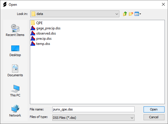
Step 18. Press Next to go to the next step. Here you will specify the destination file. Click on the folder icon to the right of the destination text field and navigate to the data folder inside your project. Once there, enter the name punx_qpe.dss in the file name text field and select Open.

Step 19. Upon returning to the wizard the destination text field will be populated, and a set of DSS path text fields will appear. For Part B use Punx and for part F use MRMS-QPE. Then press Next. The importer will show an indefinite progress bar and take several seconds to process. When it is finished it will say Import complete. You can then close the wizard and click Ok on the notification window.

Creating a Precipitation Gridset

Now that the GRIB-format precipitation data is in HEC-DSS format, it can be linked to an HEC-HMS Grid Data.

Step 20. Create a new Grid Data by using the Components menu, Create Component | Grid Data (see the beginning of this tutorial). In the dialog box that comes up, the default setting for the data type is Precipitation Gridsets. For the data we are using this is the correct choice, but if you are using any other data type make sure to verify this setting first. Set the name to MRMS-QPE and optionally set a description. Once you have specified a name and description click Create.

Step 21. Now, in the Watershed Explorer beneath a folder called Grid Data will be a folder called Precipitation Gridsets. Each grid type in HEC-HMS is distinct from one another and organized in groups. Expand this folder to find the MRMS-QPE grid dataset you just created. Click on it to select it and open the Component Editor.

Step 22. The two required settings for the gridset are the DSS Filename and DSS Pathname. First, specify the DSS Filename by clicking on the folder icon to the right of the DSS Filename text field. Then, navigate to the HEC-HMS project folder, and the data folder inside of that, where you created the punx_qpe.dss file previously using the grid data importer. Select the punx_qpe.dss file by clicking on it, and then pressing Select.

Step 23. Next you will specify the DSS Pathname by clicking on the rectangular icon to the right of the text field for the DSS Pathname. After clicking on that icon, a DSS viewer will open. Click on the first row of the DSS file and then click Set Pathname at the bottom.

Step 24. Finally, back in the Component Editor, look at the DSS Pathname text field. There are two dates in the path separated by "/" characters. Clear out both dates so that the component editor looks like below, and save by pressing the Save icon in the toolbar, or by pressing Ctrl+S. You can check out Transposing Gridded Precipitation for further reading on how the new HEC-HMS storm center calculation and transposition tools added in 4.11 can be used with the gridded storm.

Project Files

Final project files provided on the Shared Component Data Overview page

This tutorial concludes the Introduction to Shared Component Data tutorial group.