Download PDF
Download page Gage Weights Precipitation Method.
Gage Weights Precipitation Method
Return to Modeling Historical Precipitation Overview.
Last Modified: 2025-01-29 07:14:26.312
Software Version
HEC-HMS version 4.13-beta.4 was used to create this example. You can open the example project with HEC-HMS 4.13 or a newer version.
Project Files
Download the initial project files here:
Note: The initial project file is the same for the Gage Weights Precipitation, Gridded Precipitation, and Inverse Distance Precipitation tutorials. If you are completing all three tutorials, the files only need to be downloaded once.

Introduction
In this tutorial, you will associate precipitation gage data with a gage weights precipitation method in a Meteorologic Model in order to model the May 1996 precipitation event in the Mahoning Creek watershed. The precipitation gages have already been added to the HEC-HMS model. For more information on creating precipitation gage time-series, see Creating Time Series Data. The watershed has been represented using a single subbasin for the entire drainage area above the Punxsutawney stream gage.

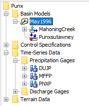
Step 1. Begin by opening up HEC-HMS 4.13-beta.2 or later. Load the project, and you will see that there are four types of elements already created: Basin Models, Control Specifications, Time-Series Data, and Terrain Data.

Step 2. Expand the Basin Models node of the Watershed Explorer Tree and select the May1996 Basin Model. You will see that this model contains two elements, a Subbasin and a Sink. You should see in the Desktop map a display that looks like the watershed above. Next, expand the Time-Series Data node of the tree and you will see that there are two types of time-series data in the model. This tutorial is concerned with the precipitation data time series. Expand that Precipitation Gages sub-node of the tree and you should see three precipitation gages.
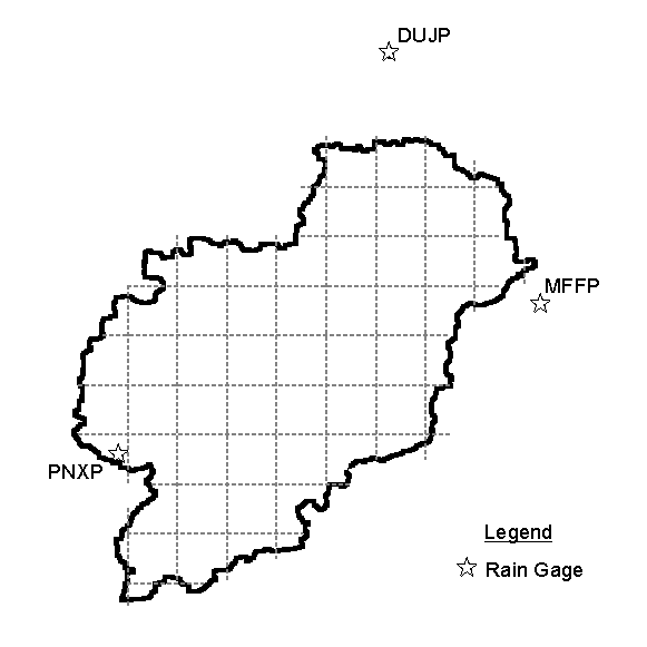
These three gages are located around the watershed and represent different observations of similar storm events. Due to the inherent variation of precipitation in space and time, these three gages are likely to observe different values of precipitation despite not being very far apart. The map below shows the location of these three stations relative to the watershed.
Step 3. Expand the gages in the Watershed Explorer to see that there is a time window associated with each of them, corresponding to the May 1996 event. You can click on the time window and then select the Graph tab in the Component Editor to see a graph of each of the gage's data for this event.

What is the time step of these precipitation gages? For a watershed of this size, is this an appropriate level of granularity for modeling a flood event?
The precipitation gages are hourly. For this size of basin, 1-hour precipitation should reasonably capture the peak rainfall intensity and therefore peak runoff. If the watershed was smaller, a finer timestep might be required.
Creating the Meteorologic Model
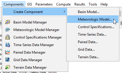
Step 4. Create a new meteorologic model by using the Components menu, then selecting Create Component > Meteorologic Model...
Step 5. For the name, enter May 1996 Gage Weights. Descriptions are optional but generally good practice. Press the Create button to create the new met model.

Step 6. There should be a new node named Meteorologic Models in the Watershed Explorer. Expand this node of the tree to see the Meteorologic Model you just created. Click on the May 1996 Gage Weights Met Model node to select it and so that you can edit it in the Component Editor.

Step 7. In the Component Editor, select the Gage Weights method for precipitation.

Step 8. Next, switch to the Basins tab and associate the Met Model with the May1996 Basin Model by toggling Include Subbasins to Yes. Save your model by pressing the save icon in the toolbar or by pressing Ctrl+S on your keyboard.

Step 9. You will see that two additional items appear beneath the May 1996 Gage Weights Met Model in the Watershed Explorer: an entry called Precipitation Gages, and then the subbasin element MahoningCreek. Expand the MahoningCreek node to see the option to set the gage weights, and then select it.

Step 10. We need to tell the Met Model which precipitation gages we want to use. Switch over to the Selections tab of the Component Editor. Here you should see the three precipitation time-series gages: DUJP, MFFP and PNXP. Enable all three of them in the Met Model by toggling the Use Gage option over to Yes. Then, save your project.

Step 11. Switch to the Weights tab of the Component Editor. Now you should see a table where the first column has the three gages you just enabled. The other two columns contain the parameters for this precipitation method, the Depth Weight and the Time Weight.
Controlling the Gage Weights Precipitation Method
Depth Weight
The depth weight controls how much each gage contributes to the total estimate for precipitation depth for a storm event. Generally this is estimated using area-average weighting, for example using Thiessen polygons. The influence of each gage on the spatial estimate of rainfall can be estimated by constructing Thiessen polygons, and then estimating the percentage of the watershed area covered by each gage's polygon, as below.

These depth weight values can be estimated using GIS by intersecting the Thiessen polygons with the watershed boundary. The estimated values serve as a starting point for estimating the contribution of each gage to the basin-averaged precipitation depth and may be adjusted during the calibration process. When there are many gages, the weight for each becomes less impactful on the result.
Step 12. For this model, enter the following depth weights that correspond to the Thiessen polygons above on the Weights tab of the Component Editor:

Time Weight
The time weight controls how much each gage contributes to the time pattern used for the storm event. In general, it is best to choose one gage located closest to the center of the watershed and give it a time weight of 1 (and the other gages 0).
Identify a side effect of averaging together time patterns that might make it harder to model a flood peak.
Primarily, averaging together the time patterns for multiple stations when the peak rainfall intensity is not coincident can result in a double-peaked hyetograph that has intensity that is overall too low.
Is it better to use a gage with a short or a long timestep for the time pattern?
Select a gage that has a fine time step so that the temporal resolution of the precipitation pattern can be well-defined. A daily gage may be available near the watershed centroid, but this will not represent sub-daily intensities. A nearby gage that is not ideally located, but has hourly or 15-minute data, will be better.
When calibrating a gage weights model, it can be beneficial to test which of the gages being used gets the time weight of 1. This can affect timing of rainfall and the shape of the overall hyetograph, and using the best gage possible for timing can improve calibration.
Step 13. For this model, set the Time Weight for PNXP (the gage inside the basin boundary) to 1, and the others to 0:

Running a Simulation
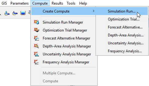
Step 14. Create a simulation run by choosing Compute menu, then Create Compute > Simulation Run.... Name the Simulation Run May 1996, select the May1996 Basin Model, select the May 1996 Gage Weights Met Model, select the May 1996 Control Specification, then press Finish.
Name the Simulation Run: May 1996
Select a Basin Model for the Simulation Run: May 1996
Select a Meteorologic Model: May 1996 Gage Weights
Select the Control Specifications: May1996
Step 15. From the Simulation Toolbar, select the May 1996 run from the drop down menu, and press the "exploding raindrop" (Compute All Elements) button to run the simulation.

Step 16. You can view the results by choosing the Results tab of the Watershed Explorer, expanding the Simulation Runs node of the tree, selecting the May 1996 Simulation Run, and clicking on the elements below it.
Project Files
Download the final project files here:
Note: The final project file is the same for the Gage Weights Precipitation, Gridded Precipitation, and Inverse Distance Precipitation tutorials. If you are completing all three tutorials, the files only need to be downloaded once.
Continue to Gridded Precipitation Method