Return to: Introduction to Point Snowmelt Calibration

Last Modified: 2023-12-11 08:54:20.283

The most complex snowmelt/accumulation modeling approach within HEC-HMS utilizes a complete energy budget to simulate the growth, evolution, and melt of a snowpack. This method is based upon the Utah Energy Budget Snow Accumulation and Melt Model (Tarboton et al 1995). This method has the ability to potentially outperform the two previously described methods when air temperature and/or net radiation are not the primary sources of energy available for snowmelt (USACE, 1998). For instance, both the Temperature Index and RTI/Hybrid methods do not implicitly include means for incorporating energy from turbulent heat transfer. However, the Energy Budget method suffers from the need for a large amount of meteorologic inputs that are not always readily available in most watersheds. Also, this method requires an iterative solution scheme and thus results in longer compute times when compared to the Temperature Index and RTI/Hybrid methods.

Parameterize the Energy Budget Snowmelt Method

Right click on the SwampAngel Basin Model and click Create Copy....
Enter SwampAngel_EB as the name and click Copy.
Expand the SwampAngel_EB node and click the SASP subbasin node.
In the Component Editor, select the Subbasin tab.
Change the Snow Method to Energy Budget.
Expand the SASP subbasin node.
Select the Energy Budget node in the project tree (or select the Snow tab).
Enter the following parameter values:
1. Leave the Precipitation Index field blank. This parameter is used to adjust the precipitation for orographic trends.
2. Rain Threshold Air Temperature (F): 32
3. Snow Threshold Air Temperature (F): 32
4. New Snow Albedo: 0.95
5. Min Snow Albedo: 0.5
6. Albedo Refresh Depth (IN): 0.25
7. Albedo Decay Coefficient Method: Fixed Value
8. Albedo Decay (HR): 600
9. Snow Thermal Conductivity (BTU/FT/DEG F/HR): 0.1
10. Liquid Water Retention Fraction: 0.25
11. Snow Hydraulic Conductivity (FT/S): 0.005
12. Soil Depth for Energy Balance (FT): 1
Right click on the Energy Budget node and select Add Elevation Band, as shown in the following image:
Expand the Energy Budget node and select Band 1.
Enter the following on the Band 1 tab:
1. Percent (%): 100
2. Elevation (FT): 11060
3. Slope (FT/FT): 0
4. Aspect (DEG): 0
5. Leave the Precipitation Index field blank. This parameter is used to adjust the precipitation for orographic trends.
6. Initial SWE (IN): 0
7. Initial Snow Depth (IN): 0
8. Initial Surface Temperature (F): 32
9. Initial Snowpack Temperature (F): 32
10. Initial Snow Albedo: 0.95
11. Initial Liquid Fraction: 0

When using the Energy Budget snowmelt method, HEC-HMS requires the modeler define the percentage of the subbasin area within each elevation band. Since we are using a single elevation band for the SASP subbasin, the Percent (%) parameter should be set to a value of 100. Also, many of the initial snow model parameters required will be set to zero because the simulation will start at the beginning of the WY when there is no snowpack.

Link the Basin Model to the Meteorologic Model

Expand the Meteorologic Models folder.
Select the WY2006 meteorologic model.
In the Component Editor, select the Basins tab.
In the SwampAngel_EB basin model row, select Yes from the drop-down menu. This links the WY2006 meteorologic model to the SwampAngel_EB basin model.
Click Save.

Create and Compute a Simulation Run

Select Compute | Create Compute | Simulation Run....
Enter WY2006_EB as the name and select Next>.
Select SwampAngel_EB Basin Model, the WY2006 Meteorologic Model, and the WY2006 Control Specifications.
Click the Finish button.
In the Toolbar, select the WY2006_EB simulation from the drop-down menu and click the Compute button:
When the simulation is complete. navigate to the Results tab.
Expand the WY2006_EB node and then expand the SASP subbasin node.
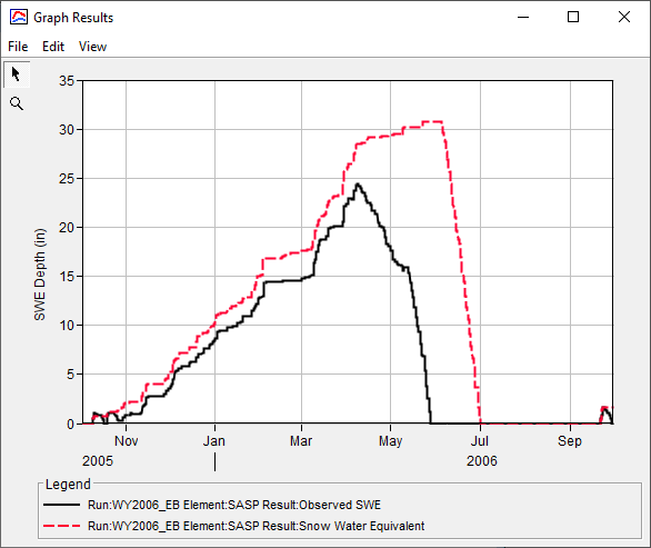
Select the Observed SWE and Snow Water Equivalent time series nodes. Click the View Graph button, as shown in the figure below. Alternatively, select the Snowmelt Graph to view Precipitation, Air Temperature, Observed SWE, and Snow Water Equivalent in the same window.

You can edit the linestyle (e.g. color, symbol, etc) of a time series by clicking Edit | Plot Properties.

Question #1: Using the initial parameter values, how does your simulated SWE compare with the observed SWE? How will you use the preliminary results to inform your calibration approach?

Simulated snow accumulation during the fall and early winter months is accelerated relative to the observed SWE time series. In addition, simulated snow continues to accumulate for nearly 2 months after peak observed SWE occurred. The simulated peak SWE is approximately 6 inches higher than the observed peak SWE magnitude.

Parameters relating to albedo tend to have a large impact on the simulated snowpack. Albedo is the reflectivity of a surface to short-wave radiation. A high albedo value means that more incident energy is reflected by the snowpack.

In addition to the New Snow Albedo, Min Snow Albedo, and Albedo Decay Coefficient, Rain Threshold Air Temperature, Snow Threshold Air Temperature, and Snow Thermal Conductivity are fairly impactful parameters. During calibration, these parameters should be changed to afford better agreement between computed and observed results.

Calibrate the Energy Budget Parameters

Revisit the Energy Balance parameters that you defined in the previous task. Modify the parameter in a systematic way and keep track of the effect of the parameter modifications on the simulated SWE. To assist with calibration, plot the Precipitation, Air Temperature, Observed SWE, and Snow Water Equivalent time series using the Snowmelt Graph.

Attempt to increase the peak SWE by modifying the Rain Threshold Air Temperature and Snow Threshold Air Temperature.
1. Try reducing the Rain Threshold Air Temperature to 30 deg F and rerun.
2. Try increasing the Rain Threshold Air Temperature to 40 deg F and rerun.
3. Try increasing the Snow Threshold Air Temperature to 35 deg F and rerun.
4. Try decreasing the Snow Threshold Air Temperature to 28 deg F and rerun.
5. Continue modifying to best match the peak SWE date and magnitude.
Attempt to improve the rate at which snow accumulates, melts, and the melt out date by modifying the New Snow Albedo and Min Snow Albedo.
1. Try decreasing the New Snow Albedo to 0.8 and rerun.
2. Try increasing the New Snow Albedo to 1.0 and rerun.
3. Try increasing the Min Snow Albedo to 0.6 and rerun.
4. Try decreasing the Min Snow Albedo to 0.1 and rerun.
5. Continue modifying the New Snow Albedo and Min Snow Albedo to best match the rate at which SWE accumulates/melts along with the computed melt out date.
Attempt to improve the rate at which snow accumulates, melts, and the melt out date by modifying the Albedo Decay Coefficient.
1. Try decreasing the Albedo Decay to 500 and rerun.
2. Try decreasing the Albedo Decay to 300 and rerun.
3. Continue modifying the Albedo Decay to best match the rate at which SWE accumulates/melts along with the computed melt out date.
Continue modifying the remaining parameters (e.g. Albedo Refresh Depth, Snow Thermal Conductivity, Snow Hydraulic Conductivity, and Soil Depth for Energy Balance) and note their impact on the computed results.
Iteratively adjust all impactful parameters to best match peak SWE magnitude, SWE melt rate, and melt out date.

Question #2: Which parameters had the largest impact on the simulated SWE?

The New Snow Albedo and the Albedo Decay Coefficient values had the largest impact on the rate of snow accumulation and melt. A high New Snow Albedo means that more incident energy is reflected, resulting in prolonged snow accumulation. The Albedo Decay Coefficient is the coefficient used in an exponential decay function to describe the decrease in albedo as the snowpack ages. A high Albedo Decay Coefficient means that the snowpack albedo decays slowly. Reducing these parameters shifted the simulated peak SWE to earlier in the season and caused snowmelt to beging earlier.

Question #3: What is the final set of parameters used to simulated SWE at the Swamp Angel Study Plot?

The calibrated Energy Budget parameters are shown in the table below. These values produced a NSCE of 0.98 and a PBIAS of -3%. In addition, the simulated date of peak SWE is within 24 hrs of the observed date of peak SWE. The simulated peak SWE of 25.6 inches is very close to the observed peak SWE of 24.4 inches.

The Snow Threshold Air Temperature was reduced from 32 deg F to 31 deg F. The lower Snow Threshold Air Temperature caused precipitation to fall as rain, rather than as snow, in April. This caused snow accumulation to stop earlier in the season and reduced the simulated peak SWE amount.
The New Snow Albedo was reduced from 0.95 to 0.75. This caused the snowpack to absorb more radiation which initiated melt earlier in the season.
The Albedo Refresh Depth is the depth of snow required to reset the snowpack albedo to the New Snow Albedo. This value was reduced from 0.25 inches to 0.2 inches, meaning that the snow albedo was reset to 0.875with 0.2 inches of snow.
The Albedo Decay Coefficient was reduced from 600 hr to 550 hr. This caused the simulated rate of melt to match the observed rate of melt.
The Liquid Water Retention Fraction was reduced from 0.25 to 0.01. The Liquid Water Retention Fraction is used to compute the portion of energy content held as liquid water in the snowpack. Reducing the Liquid Water Retention Fraction reduces the energy content of the snowpack. As a result, less atmospheric energy is needed to raise the temperature of the snowpack to the freezing point and initiate melt.
The Effective Thermal Ground Depth was reduced from 1 ft to 0.1 ft. This value represents the depth of soil that thermally interacts with the snowpack.