Download PDF
Download page Creating a Complex 2D Flow model within HEC-HMS.
Creating a Complex 2D Flow model within HEC-HMS
HEC-HMS version 4.10 was used to created this tutorial. You will need to use HEC-HMS version 4.10, or newer, to open the project files.
Introduction
The new 2D Diffusion Wave transform method within HEC-HMS version 4.7 explicitly routes excess precipitation throughout a subbasin element using a combination of the continuity and momentum equations. As such, this new transform method can be used to simulate the non-linear movement of water throughout a subbasin when exposed to large amounts of excess precipitation. A tutorial detailing this use case is contained here: Creating a Simple 2D Flow Model within HEC-HMS.
In addition to routing excess precipitation, the new 2D Diffusion Wave transform method can be used to accurately simulate the movement of water in both defined stream channels as well as overbank areas. This guide provides step-by-step instructions that can be used to modify an existing HEC-HMS project to accurately simulate the movement of water in a complex area using the new 2D Diffusion Wave transform method.
Truckee River Watershed
This example uses the Truckee River watershed which originates at the outlet of Lake Tahoe in California. The Truckee River flows for over 100 miles and eventually empties into Pyramid Lake in Nevada. Major population centers within the Truckee River watershed include the cities of Truckee, CA, Reno, and Sparks, NV with a total population greater than 350,000 (as counted during the 2010 census). Numerous state and federal water supply and flood risk management projects have been constructed within this watershed. Several major federally-constructed projects include Martis Creek Dam, Prosser Creek Dam, Stampede Dam, and Boca Dam, as shown in Figure 1.

The Truckee River upstream of the United States Geological Survey (USGS) gage at Reno, NV (10348000; https://waterdata.usgs.gov/nv/nwis/inventory/?site_no=10348000&agency_cd=USGS) drains over 1000 sq mi of rugged terrain within the Sierra Nevada mountains. Upstream of this gage, numerous peaks in excess of 10,000 ft are present along with extremely steep channels (slopes > 50 ft/mi) and incised canyons. However, in the vicinity of Reno and Sparks, NV, channel slopes reduce to nearly 1 ft/mi and a floodplain several miles wide forms. Additionally, the Truckee River receives two tributaries: 1) Steamboat Creek from the south and 2) North Truckee Ditch from the north. Downstream of the USGS gage at Vista, NV (10350000; https://waterdata.usgs.gov/nwis/uv?site_no=10350000), the floodplain contracts and the Truckee River enters another steep canyon, as shown in Figure 2.

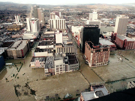
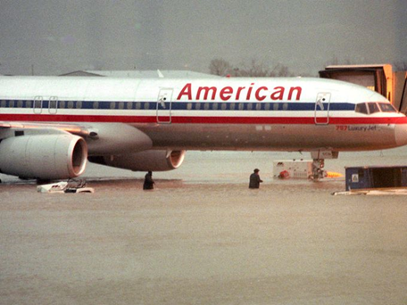
While the Truckee River provides a major source of water for its nearby inhabitants, the river is also prone to significant flooding. Substantial damage to urban areas has occurred during large scale and widespread rain-on-snow flood events in January 1997, December 2005 - January 2006, and January - February 2017 (amongst others). The extent of flooding during January 1997 within downtown Reno and at the Reno-Tahoe Airport are shown in Figures 3 and 4, respectively.
Existing HEC-HMS Project
An HEC-HMS was used to simulate the precipitation-runoff processes throughout the Truckee River watershed. This model, which was originally built as part of a Corps Water Management System (CWMS) implementation, was modified to route excess precipitation with the Modified Clark unit hydrograph method and route streamflow using both the Muskingum-Cunge and Modified Puls channel routing methods. This model is detailed here: Modeling Rain-on-Snow Events.
The January 1997 flood event (spanning from late December 1996 through early January 1997) was simulated with this model. The results upstream of the Reno gage were found to adequately reproduce observed streamflow, reservoir inflow/outflow/pool elevation, and snow data, as shown in Figure 5. However, computed streamflow was found to deviate from observed streamflow at the Vista gage, as shown in Figure 6. Specifically, computed streamflow at the Vista gage arrived earlier and was more peaked than the observed data suggested.


These inaccuracies are due to: 1) the complex hydraulic interactions in and around the cities of Reno and Sparks, NV and 2) the hydrologic routing simplifications within the existing HEC-HMS model. During this flood (and other large floods), streamflow exceeded the channel capacity of the Truckee River and Steamboat Creek and began to spread throughout the very wide floodplain. Also, the large amount of runoff was constricted by the natural topography downstream of the Vista gage. These complex hydraulic scenarios cannot be accurately simulated using hydrologic routing. To more accurately route water within the area of interest in and around the cities of Reno and Sparks, NV during large floods, the existing HEC-HMS model was modified to use the new 2D Diffusion Wave transform. The following sections detail the processes which were used to update this model.
Input Data
Multiple pieces of input data were needed to accurately simulate the movement of water within the area of interest for the time period of interest. These data are detailed in the following sections.
Streamflow
Streamflow data for major USGS gages within the Truckee River watershed was downloaded from the USGS National Water Information System (NWIS) database using plugins available within HEC-DSSVue. These plugins import data from the USGS NWIS database and create new time series records within a DSS file. Specifically, the instantaneous peak streamflow, daily average flow, and 15- or 60-min flow time series for December 1996 - January 1997 were downloaded.
Terrain
A 1/3rd arc-second digital elevation model (DEM) encompassing the entire Truckee River watershed was downloaded from the USGS National Map Viewer: https://apps.nationalmap.gov/viewer/. Within the area of interest, 1/3rd arc-second equates to a horizontal resolution of approximately 10 meters. The NED 10m DEM was used to make modifications to the subbasin delineations within the existing HEC-HMS project. The NED 10m DEM was clipped using a buffered polygon that surrounded the Truckee River watershed, projected to the Albers Equal Area Conic coordinate system, and the vertical units were converted to feet. The resultant NED 10m DEM is shown in Figure 7.

A 1 meter horizontal resolution DEM encompassing the area of interest in and around the cities of Reno and Sparks, NV was also downloaded from the USGS National Map Viewer. The NED 1m DEM was used to populate properties within the two-dimensional (2D) mesh within the area of interest. The NED 1m DEM was clipped using a buffered polygon that surrounded the area of interest, projected to the Albers Equal Area Conic coordinate system, and the vertical units were converted to feet. The resultant DEM is shown in Figure 8.

Land Use
Land use classifications were downloaded from the Multi-Resolution Land Characteristics Consortium: https://www.mrlc.gov/data?f%5B0%5D=category%3Aland%20cover. The National Land Cover Database (NLCD) 2016 version represents the most up-to-date nationwide source for land cover classifications. The NLCD 2016 classifications were used to designate roughness values within the 2D mesh. The land use classifications within the area of interest are shown in Figure 9.

Hydrography
Stream centerlines from the National Hydrography Data Plus (NHDPlus) data set were downloaded: https://www.usgs.gov/core-science-systems/ngp/national-hydrography/nhdplus-high-resolution. The stream centerlines were clipped using a buffered polygon that surrounded the area of interest. The stream centerlines were used to designate stream channels (which have lower roughness values relative to the overbank areas) within the 2D mesh.
Precipitation
Hourly gaged precipitation for the time period of interest was downloaded from the National Centers for Environmental Information (NCEI): https://www.ncdc.noaa.gov/. GageInterp was then used to create hourly precipitation grids which captured the temporal and spatial resolution of precipitation throughout the Truckee River watershed: https://www.hec.usace.army.mil/training/CourseMaterials/Mongolia_Workshop/gageInterpUserManual.pdf.
Parameter-elevation Regressions on Independent Slopes Model (PRISM) precipitation for the time period of interest was also downloaded: https://prism.oregonstate.edu/. In general, this data represents the spatial and temporal distribution of precipitation much better than the gage precipitation (and resultant grids created by gageInterp). The PRISM data was first projected to the Standard Hydrologic Grid (SHG), clipped to the area of interest, and converted to DSS format using Vortex: https://github.com/HydrologicEngineeringCenter/Vortex. The PRISM data was used to "correct" the gageInterp output at a daily time step. In essence, each grid cell within the gageInterp grids was adjusted to to equal the corresponding grid cell within the PRISM data set.
Temperature
Hourly gaged temperature for the time period of interest was downloaded from the NCEI. GageInterp, along with a lapse rate of 4.6 deg C / 1000 meter of elevation, was then used to create hourly temperature grids. This lapse rate was developed using prevailing temperatures from nearby gages and their respective elevations during the time period of interest.
Snow Data
Antecedent snow water equivalent (SWE) for 27 December 1996 was developed using gage information from NCEI and Snow Telemetry (SNOTEL) stations that are maintained by the Natural Resources Conservation Service (NRCS).
Modifications to the Existing HEC-HMS Project
To utilize the 2D Diffusion Wave transform within HEC-HMS, the subbasin elements of interest must be georeferenced. New GIS features have been recently added to HEC-HMS to aid in this process. These features allow the user to create an HEC-HMS model from scratch, georeference existing basin model elements using shapefile information, and/or update subbasin and reach delineations.
A copy of the existing January 1997 flood basin model was created (called "Jan_1997_2D"), the previously mentioned NED 10m terrain data was added to the project, and the NED 10m terrain data was associated with the copied basin model. Next, the HEC-HMS GIS tools were then used to merge the three subbasin elements that represent the land surface processes throughout the area of interest into one (called "RenoSparks"). Also, the three reach elements representing the Truckee River, Steamboat Creek, and North Truckee Ditch within the area of interest were removed. The resultant layout is shown in Figure 10.

The "RenoSparks" subbasin was then exported as a shapefile using the GIS | Export Georeferenced Elements tool. Finally, every subbasin except "RenoSparks" was set to use the Structured discretization method and grid cells were computed by clicking GIS | Compute Grid Cells.
Choosing Modeling Processes and Estimating Initial Parameter Values
The Gridded Temperature Index snowmelt, Simple canopy, Deficit and Constant loss, 2D Diffusion Wave, and Linear Reservoir baseflow methods were selected for use within this new subbasin. Initial estimates for each parameter within the aforementioned methods were then made using area weighted averages from the subbasins which were merged together and are shown in the following tables:
Gridded Temperature Index Snowmelt Parameter | Value |
|---|---|
| Initial SWE Grid | Jan_1997_iSWE |
| Initial CC Grid | zeroCC |
| Initial Liquid Grid | zeroLWC |
| Initial CC ATI Grid | zeroCCATI |
| Initial Melt ATI Grid | zeroMRATI |
| PX Temperature (deg F) | 30 |
| Base Temperature (deg F) | 30 |
| Wet Melt Method | Constant Value |
| West Meltrate (in / Deg F - day) | 0.1 |
| Rain Rate Limit (in / day) | 0.1 |
| ATI-Meltrate Coefficient | 0.98 |
| Dry Melt Method | ATI-Meltrate Function |
| ATI-Meltrate Function | Mt_Rose_Ski_Area_much_slower |
| Cold Limit (in / day) | 0.2 |
| ATI-Coldrate Coefficient | 0.35 |
| ATI-Coldrate Function | Averaged |
| Water Capacity (%) | 3 |
| Groundmelt (in / day) | 0 |
Simple Canopy Parameter | Value |
|---|---|
| Initial Storage (%) | 0 |
| Maximum Storage (in) | 0 |
| Crop Coefficient | 1.0 |
| Evapotranspiration | Only Dry Periods |
| Update Method | Simple |
Deficit and Constant Loss Parameter | Value |
|---|---|
| Initial Deficit (in) | 2.45 |
| Maximum Deficit (in) | 7.36 |
| Constant Rate (in/hr) | 0.31 |
| Directly Connected Impervious Area (%) | 9.3 |
2D Diffusion Wave Parameter | Value |
|---|---|
| Implicit Weighting Factor (theta) | 1.0 |
Water Surface Tolerance (ft) | 0.001 |
| Volume Tolerance (ft) | 0.001 |
| Max Iterations | 20 |
| Max Courant Number | 1.0 |
| Max Time Step (sec) | 60 |
| Warm Up Period (hr) | 72 |
| Warm Up Period Fraction | 0.5 |
| Number of Cores | 4 |
Linear Reservoir Baseflow Parameter | Value |
|---|---|
| Number of Layers | 2 |
| GW 1 Initial (cfs / mi2) | 0 |
| GW 1 Fraction | 0.22 |
| GW 1 Coefficient (hr) | 36.2 |
| GW 1 Steps | 1 |
| GW 2 Initial (cfs / mi2) | 0.5 |
| GW 2 Fraction | 0.22 |
| GW 2 Coefficient (hr) | 841.9 |
| GW 2 Steps | 1 |
Creating a Mesh and Boundary Conditions within HEC-RAS
Currently, users must create a 2D mesh and any associated normal depth, flow, stage, and/or rating curve boundary conditions within HEC-RAS (version 5.0.7 or newer) and then import to HEC-HMS. In the future, users will be able to create and modify both 2D meshes and boundary conditions entirely within HEC-HMS.
To create a 2D mesh within HEC-RAS, a new project was started and an empty, new Geometry file (called "base") was created. Next, RAS Mapper was opened and the previously mentioned NED 1m terrain data was imported and associated with the new geometry. Then, a single 2D Area (called "RenoSparks") was created using the subbasin shapefile, which was previously exported from HEC-HMS. Breaklines were used to align cell faces with prominent topographic features like roadways and embankments. Computation points were then created within the HEC-RAS | Geometric Data editor using a 500 ft x 500 ft spacing. Finally, three Boundary Condition lines were created at the Reno gage location (called "Truckee_inflow"), Short Lane gage location (called "Steamboat_inflow"), Spanish Springs gage location (called "NTruckeeDt_inflow"), and Vista gage location (called "Truckee_outflow"). The 2D mesh, breaklines, and boundary condition lines are shown in Figure 11.

In order to better simulate the movement of water throughout the area of interest, a spatially distributed Manning's n Layer was created within RAS Mapper. To allow for faster movement of water through defined stream channels, a buffered polygon layer surrounding the previously described NHD streams was created and imported to RAS Mapper. Then, a new Manning's n layer was created by combining the previously mentioned NLCD 2016 land use classifications and the buffered streams polygon layer; the buffered streams polygon layer was placed at the highest hierarchy (i.e. overrides the NLCD 2016 land use classifications). Initial estimates for Manning's n were assigned using the following table:
Land Cover Classification | Manning's n |
|---|---|
| Streams | 0.06 |
| Barren Land Rock/Sand/Clay | 0.06 |
| Cultivated Crops | 0.1 |
| Deciduous Forest | 0.1 |
Developed, High Intensity | 0.08 |
| Developed, Medium Intensity | 0.07 |
| Developed, Low Intensity | 0.06 |
| Developed, Open Space | 0.06 |
| Emergent Herbaceous Wetlands | 0.1 |
| Evergreen Forest | 0.1 |
| Grassland/Herbaceous | 0.1 |
| Mixed Forest | 0.1 |
| Open Water | 0.06 |
| Pasture/Hay | 0.1 |
| Shrub/Scrub | 0.1 |
| Woody Wetlands | 0.1 |
This new Manning's n Layer was then associated with the geometry and is shown in Figure 12.

A new Unsteady Flow file was then created and five boundary conditions were parameterized: 1) 0.1 inch of spatially and temporally uniform precipitation applied to the 2D mesh, 2) a flow hydrograph using an energy grade slope of 0.008 ft/ft for the "Truckee_inflow" boundary condition line, 3) a flow hydrograph using an energy grade slope of 0.007 ft/ft for the "Steamboat_inflow" boundary condition line, 4) a flow hydrograph using an energy grade slope of 0.007 ft/ft for the "NTruckeeDt_inflow" boundary condition line, and 5) a friction slope of 0.0002 ft/ft for the "Truckee_outflow" boundary condition line; the precipitation depth is meaningless as it is only used to allow for a successful simulation. Next, a new Unsteady Plan was created and the previously described geometry and unsteady flow files were selected. A valid simulation time window and computation settings were set to allow for a successful simulation. Finally, the unsteady flow simulation was computed, which generated an Unsteady Plan HDF file, which has an extension of ".p##.hdf" where "p##" corresponds to the specific plan of interest. This file contains the computational mesh and boundary condition line information which are currently needed by HEC-HMS.
Importing the Mesh and Boundary Conditions to HEC-HMS
Following the generation of the Unsteady Plan HDF file within HEC-RAS, the 2D mesh and associated boundary condition line information was imported to HEC-HMS using the HDF File Import Wizard. This wizard can be accessed within HEC-HMS by clicking File | Import | HEC-RAS HDF File... On the first panel, the Unsteady Plan HDF file was selected, as shown in Figure 13.

On the second panel, the "Jan_1997_2D" basin model was selected, as shown in Figure 14.

On the third panel, the "RenoSparks" subbasin was selected, as shown in Figure 15.

On the fourth panel, the "RenoSparks" 2D Mesh was selected, as shown in Figure 16.

Upon clicking Finish, the 2D mesh was imported, the "RenoSparks" subbasin's Discretization was changed to Unstructured, and four 2D Connection nodes (called "Truckee_inflow", "Steamboat_inflow", "NTruckeeDt_inflow", and "Truckee_outflow") were added. Also, the 2D Mesh and 2D Connections are shown within the Map Panel, as shown in Figure 17. Note: you may need to click View | Map Layers and turn on the Discretization and 2D Connection map layers.

Connecting Elements
Within HEC-HMS, 2D Connections are used to supply boundary conditions as well as link other elements to/from the 2D mesh. As such, existing elements within the HEC-HMS project were connected to the newly imported 2D Connections to supply inflow and receive outflow:
- The existing "Reno" junction was connected to the "Truckee_inflow" 2D Connection by opening the "Reno" Component Editor and selecting the "Truckee_inflow" 2D Connection within the Downstream drop down menu
- The existing "ShortLane" junction was connected to the "Steamboat_inflow" 2D Connection by opening the "ShortLane" Component Editor and selecting the "Steamboat_inflow" 2D Connection within the Downstream drop down menu
- The existing "SpanishSprings" junction was connected to the "NTruckeeDt_inflow" 2D Connection by opening the "SpanishSprings" Component Editor and selecting the "NTruckeeDt_inflow" 2D Connection within the Downstream drop down menu
- The "Truckee_outflow" 2D Connection was connected to the existing "Vista" junction by opening the "Truckee_outflow" Component Editor and selecting the "Vista" junction within the Downstream drop down menu
Next, the 2D Connections were parameterized:
- The "Truckee_inflow" 2D Connection type was set to Flow Hydrograph, an Energy Grade Slope of 0.008 ft/ft was set, and a Ratio of Subbasin Baseflow of 0.0 was entered
- The "Steamboat_inflow" 2D Connection type was set to Flow Hydrograph, an Energy Grade Slope of 0.007 ft/ft was set, and a Ratio of Subbasin Baseflow of 0.0 was entered
- The "NTruckeeDt_inflow" 2D Connection type was set to Flow Hydrograph, an Energy Grade Slope of 0.007 ft/ft was set, and a Ratio of Subbasin Baseflow of 0.0 was entered
- The "Truckee_outflow" 2D Connection type was set to Normal Depth, a Friction Slope of 0.0002 ft/ft was set, and a Ratio of Subbasin Baseflow of 1.0 was entered
The Ratio of Subbasin Baseflow is defined as the ratio of baseflow generated within the "RenoSparks" subbasin that will reach each 2D Connection. In this case, all baseflow generated within the "RenoSparks" subbasin was set to reach the "Truckee_outflow" 2D Connection, as shown in Figure 18.

Creating a Simulation Run within HEC-HMS
A simulation run within HEC-HMS requires a Basin Model, Meteorologic Model, and Control Specification. The existing "Jan_1997" meteorologic model was used. This meteorologic model was set to use the Gridded Precipitation, Gridded Hamon evapotranspiration, and Gridded Temperature methods. The existing "Jan1997" Control Specification was selected and a Start Date, Start Time, End Date, End Time, and Time Interval of "27Dec1996", "06:00", "15Jan1997", "06:00", and "1 Hour" was used, respectively. Finally, a new Simulation Run (called "Jan_1997_2D") was created. The previously mentioned Basin Model, Meteorologic Model, and Control Specifications were selected and the simulation run was computed.
Investigating the Results
Once the simulation run was successfully computed, results for the "Vista" junction were plotted and are shown in Figure 20.

As is evident in this figure, the computed results match the observed streamflow much better than the results which were previously presented in Figure 6. Also, time series for each 2D Connection were plotted and investigated, as shown in Figure 21.

Finally, spatial variables like SWE, cumulative precipitation, hydraulic depth, water surface elevation, and velocity were investigated. A tutorial showing how to turn on and view spatial results can be found here: Viewing Spatial Results for a Structured Discretization. As shown in Figure 22, the spatial results indicate streamflow exceeding the Truckee River channel capacity starting just downstream of the Reno gage and spreading throughout the floodplain. Also, the backwater effects caused by the natural topographic constriction in the vicinity of the Vista gage results in reduced average cell velocities and excessive hydraulic depths throughout the area of interest, as shown in Figure 23.
The computed hydraulic depths were compared with observations of both depth and inundation extent, as shown in Figure 24, and were found to compare well.


Videos of hydraulic depth, average cell velocity, and water surface elevation within the area of interest are shown below. Also, videos of cumulative precipitation and SWE throughout the entire Truckee River watershed are shown below.
At this point, the modeler can make changes to the loss, baseflow, and 2D Connection methods/parameterizations to provide a better response throughout the watershed. However, HEC-HMS does not currently allow the user to modify Manning's n values within a 2D mesh. This must be accomplished within HEC-RAS by generating a new Unsteady Plan HDF file and importing to HEC-HMS. In the future, users will be able to create and modify Manning's n Layers entirely within HEC-HMS in addition to many new features related to 2D flow.
HEC-HMS Project
The completed HEC-HMS project can be downloaded here: Truckee_River.zip.
References
NHD: Buto, S.G., and Anderson, R.D., 2020, NHDPlus High Resolution (NHDPlus HR)---A hydrography framework for the Nation: U.S. Geological Survey Fact Sheet 2020-3033, 2 p., https://doi.org/10.3133/fs20203033.
MRLC: https://www.mrlc.gov/data?f%5B0%5D=category%3Aland%20cover
3DEP: https://www.usgs.gov/core-science-systems/ngp/3dep/
USGS NWIS: https://waterdata.usgs.gov/nwis
NOAA NCEI: https://www.ncdc.noaa.gov/
PRISM: PRISM Climate Group, Oregon State University, http://prism.oregonstate.edu, accessed August 2020.