Download PDF
Download page Bulletin 17C Flow-Frequency augmented by Precipitation-Frequency with HEC-HMS.
Bulletin 17C Flow-Frequency augmented by Precipitation-Frequency with HEC-HMS
Overview
This tutorial provides an example of using precipitation-frequency estimates in conjunction with an HEC-HMS model to help inform the upper end of a flow frequency curve. HEC-SSP version 2.3 beta.1 and HEC-HMS version 4.10 beta.1 were used to create this example.
Download a copy of the HEC-SSP project here – French_Creek_SSP.zip
Download a copy of the HEC-HMS project here – French_Creek_HMS.zip
Introduction
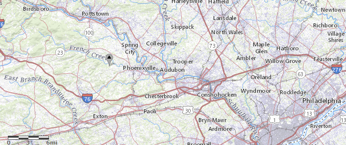
The site used for this example is French Creek near Phoenixville, Pennsylvania. The goal is to produce an instantaneous peak annual maximum flow-frequency curve at this site, with the focus on the frequency range from 1% AEP (100-year) to 0.1% AEP (1000-year) for floodplain management applications. The USGS gage at this site includes 52 years of record from 1969-2021. The site has a drainage area of 59 square miles, and there are no dams upstream. Urban development in the basin is relatively limited as well. Flood-producing mechanisms are mostly purely rainfall-driven, though some annual maximum peaks have occurred as a result of rain-on-snow events. This site should be an ideal candidate for this type of analysis, but we will see that even for an ideal site, the process is rarely straightforward.
EM 1110-2-1417 contains guidance on performing flood-frequency analysis. It notes that different methods can be adopted depending on the purpose of the analysis. In this example, we will explore two different methods and discuss how they could be combined:
- Statistical analysis of observed streamflow data (Bulletin 17C analysis)
- Event-type precipitation-runoff analysis with hypothetical storms (precipitation-frequency combined with HEC-HMS model)
EM 1110-2-1417 notes "In many cases, frequency estimates should be developed by several independent techniques. Different segments of the adopted frequency curve may be derived from different sources depending on the basis for, and reliability of, the individual estimates." Observed streamflow records are often used for the more common segment of the flow-frequency curve, and precipitation-frequency in conjunction with HEC-HMS modeling can be used to inform the more extreme upper end of the frequency curve. This is often done because the record lengths of observed peak flows are relatively short. While the record length of precipitation records are only a little longer, the power of a precipitation-frequency analysis is that it leans on regionalization, using data at a vast array of nearby precipitation gages to develop frequency estimates. This can greatly reduce uncertainty at the extreme ends of the precipitation-frequency curve, and is known as "trading space for time." In this example, we will see if this approach makes sense here.
Bulletin 17C using observed flow data only
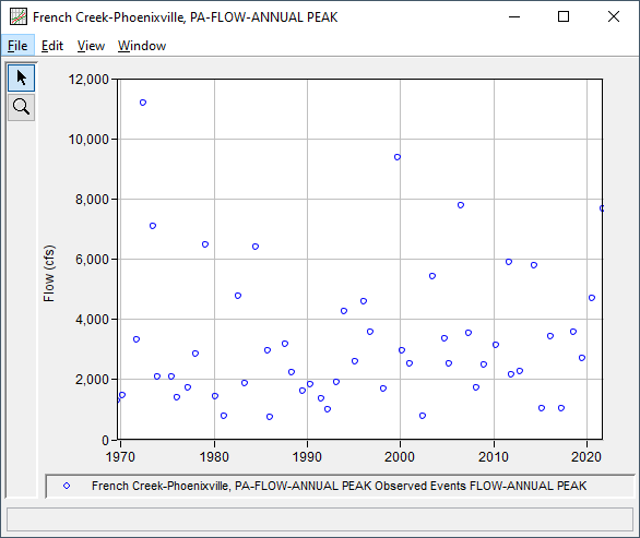
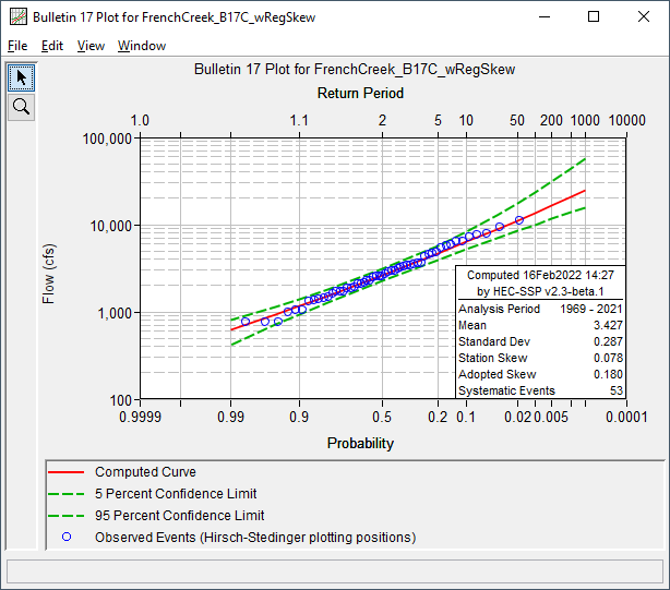
A Bulletin 17C flow-frequency analysis based on observed streamflow data is performed first. See this tutorial for an example of performing a Bulletin 17C analysis: SSPTutorialsGuides:Task 4. Bulletin 17C. While there may some influences from mixed population effects here (hurricanes vs rain on snow events), they appear to be relatively minor and will be ignored for this example. The observed record from 1969-2021 forms the backbone of the analysis. Other nearby gages with longer records were investigated to see if record extension techniques could be used to add additional flow estimates earlier in time, but no suitable long-term gage was found. For an example of this process, refer to this tutorial: Task 1. Create a new HEC-SSP Study and Import Data. A regional skew analysis was available (https://pubs.er.usgs.gov/publication/sir20195094), giving a regional skew of 0.35 with a mean square error (MSE) of 0.181. As such, the weighted skew option was used. Since the station skew was fairly similar to the regional skew, incorporating regional skew only modestly changed the results. While additional research should be undertaken to investigate historic floods before the gage records exist, this step was not taken for this example for simplicity. The peak flow record and the flow-frequency curve using Bulletin 17C is shown below.
HEC-HMS Model overview
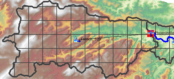
An HEC-HMS model has previously been developed for this basin. A single subbasin is used to represent the drainage area upstream of Phoenixville. The model was calibrated to the January 1996 event and the June 2006 event, using gridded inputs. Calibration plots are shown below, as well as a table summarizing the key basin model parameters used.
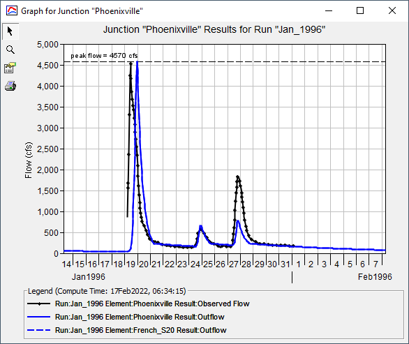
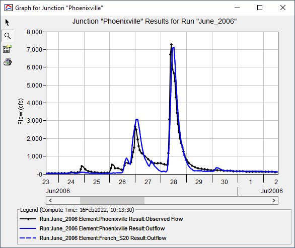
| Basin Parameter | January 1996 | June 2006 |
|---|---|---|
| Loss (Deficit and Constant) | ||
| Initial Deficit (in) | 1 | 2.8 |
| Constant Rate (in/hr) | 0.11 | 0.09 |
| Transform (Mod Clark Unit Hydrograph) | ||
| Time of Concentration (hr) | 5.56 | 4.9 |
| Storage Coefficient (hr) | 9.81 | 4.9 |
| Baseflow (Recession) | ||
| Recession Constant | 0.90 | 0.85 |
| Ratio to Peak | 0.05 | 0.025 |
Precipitation-Frequency Information
NOAA Atlas 14 is the primary source for precipitation-frequency information for most of the U.S. It provides point estimates of precipitation for various frequencies (return intervals). The 6-hour, 1% AEP (100-year) point-precipitation map is shown below.
https://hdsc.nws.noaa.gov/hdsc/pfds/pfds_map_cont.html?bkmrk=pa
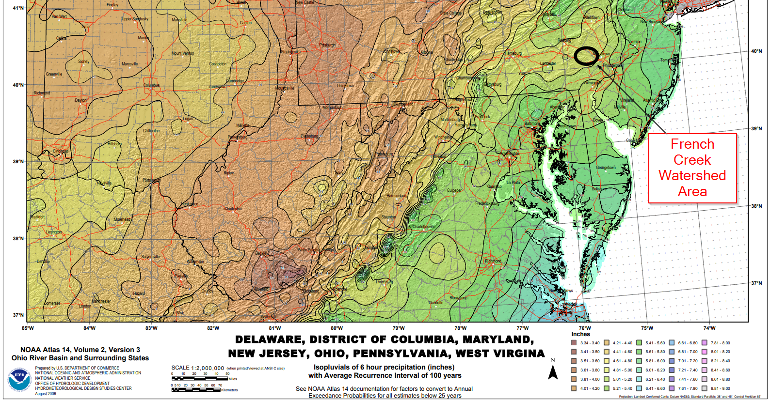
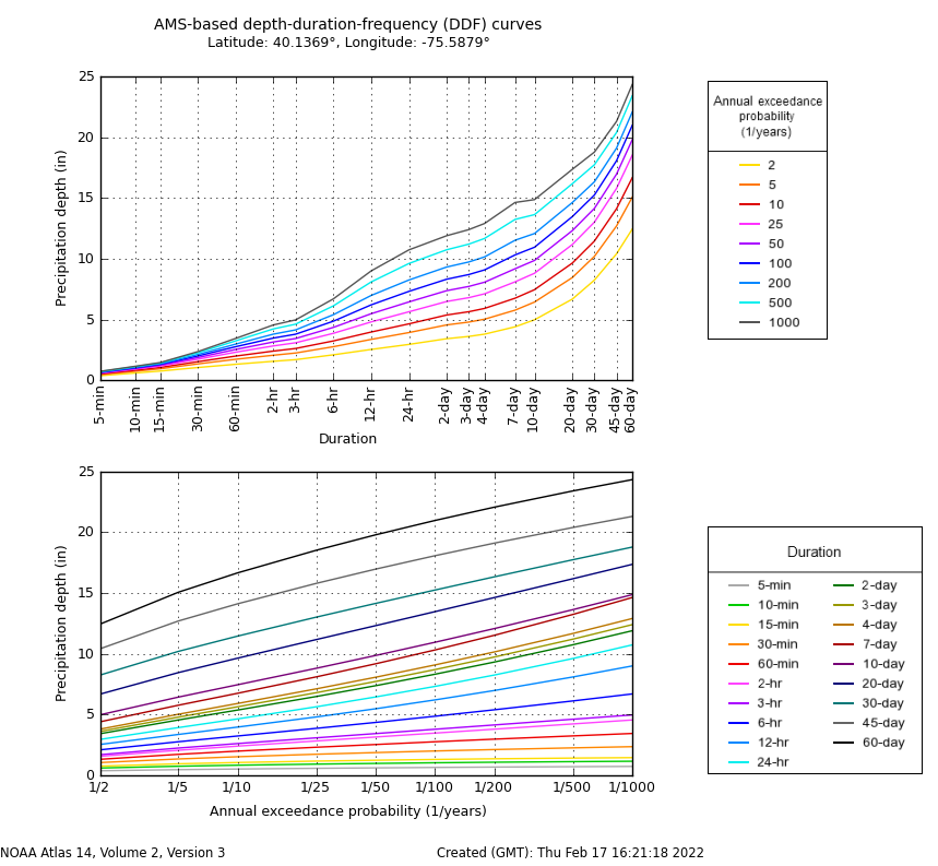
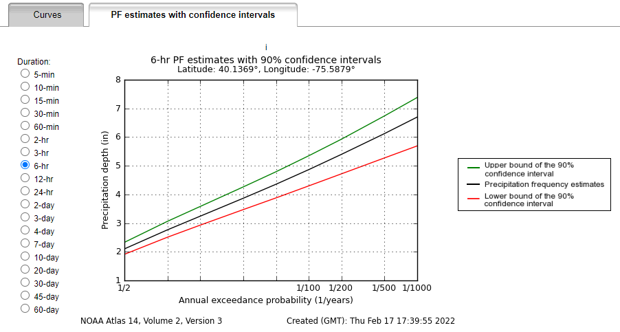
The map shows that there is not much spatial variability in the point precipitation-frequency curves in the small French Creek watershed. Therefore, the spatial distribution of precipitation will likely not be a very influential component. If a larger watershed area was being analyzed, spatial patterns of precipitation would become more important. The precipitation-frequency curves from NOAA Atlas 14 at a point inside the French Creek watershed area are shown below for context:
Using Precipitation-frequency information with HEC-HMS
Per EM 1110-2-1417, "Although the NOAA rainfall criteria associate frequency with depth, it does not follow that the same frequencies should be associated with design storms or the calculated flood-runoff". In other words, the 100-year precip event does not always correspond to a 100-year runoff event. Peak flows are a function of many factors other than just precipitation, including:
- Precipitation amount
- Storm duration
- Temporal pattern of storm
- Spatial pattern of storm
- Antecedent conditions, such as starting snow or soil moisture
- Temperature sequence (for snowmelt contributions)
- Basin loss rates and computational method
- Basin unit hydrograph parameters and computational method
- Basin baseflow parameters and computational method
- Reservoir regulation effects (when applicable)
Per EM 1110-2-1417: "Because of the uncertainty of the frequency of design-storm runoff, it is best to utilize statistically based frequency information (...) wherever possible to 'calibrate' the exceedance frequency to associate with particular combinations of design storms and loss rates." Observed flow estimates are immensely valuable, since they already include the interrelated effects of all these components working together. In contrast, when using a rainfall-runoff model paired with precipitation-frequency curves, all of these individual components must be addressed.
In this section of the tutorial, we will use the HEC-HMS model paired with the precipitation-frequency curves. The Hypothetical Storm meteorologic model paired with the Frequency Analyses compute method will be primarily used for this example. Refer to this tutorial for an example of creating the Hypothetical Storm meteorologic model: Creating-a-hypothetical-storm-precipitation-method. A video explaining this method can be found here:
Another commonly-used approach in this situation is the Frequency Storm meteorological model. This approach is known as a "balanced hyetograph" approach. Per EM 1110-2-1417, in a balanced hyetograph: "the depth associated with each duration interval of the storm satisfies the relation between depth and duration for a given frequency. For example, for a 1 percent-chance (100-year) 24-hr storm, the depth for the peak 30-min, 1-hr, 2-hr, ..., 24-hr durations would each equal the 1 percent chance for that duration. Although such storms do not preserve the random character of natural storms, use of a balanced storm ensures an appropriate depth (in terms of frequency), regardless of the time-response characteristics of a particular river basin". This approach is often used for design applications, but the poor comparisons to observed storms do not lend this method well to flow-frequency analysis when observed precipitation and flow data is available. The Frequency Storm method is not used in this tutorial.
Storm Duration
From EM 1110-2-1417: "(...) the duration is generally chosen to equal or exceed the time of concentration for a watershed." A typical estimate for storm duration is to pick a duration that is slightly longer than the time of concentration of the watershed. In our example, the time of concentration is about 5 hours, so we'll pick a storm duration of 6 hours to start. In a more detailed study, a critical duration analysis would be performed. In general terms, this analysis would correlate various durations of precipitation with the instantaneous peak flow at Phoenixville for observed events, and choose the duration with the highest correlation.
Precipitation Amount
Precipitation-frequency curves were sourced from NOAA Atlas 14. The point precipitation estimate is shown below with uncertainty bounds for a point inside the French Creek basin. Note that the 90% confidence interval is relatively narrow–even for the 1/1000 event, the upper uncertainty bound is less than an inch higher than the best estimate. This suggests relatively high confidence in the precipitation-frequency curves.
The estimates direct from NOAA Atlas 14 are for a single point. However, it is well established that average precipitation intensity decreases as the area of a storm increases. A depth-area reduction factor is used to account for this relationship. If a depth-area reduction factor were not applied, the precipitation for a given frequency event would be overestimated. The area reduction factors from TP-40 are used for this example. For a storm area of 59 square miles, the area reduction factor is about 90%. For instance, the point precipitation for the 5-year, 6 hour event is 2.77 inches from NOAA Atlas 14. After applying the area reduction factor, the basin-average precipitation that will be applied in HMS is 2.50 inches. This factor is not very consequential in this small drainage area, but the area-reduction factors become more critical for larger watersheds.
Temporal Pattern
The temporal pattern of the storm determines when the precipitation falls through time. There are a wide variety of potential temporal patterns: observed storms can be used, or patterns from NOAA Atlas 14 can be used. The patterns from NOAA Atlas 14 are described with two parameters: the quartile of the storm with heaviest precipitation, and the percentile of the precipitation within that quartile. For instance, the 6-hour, 2Q, 10% pattern means that the precipitation is heaviest from hour 1.5 to 3, and 10% of the storms used to develop NOAA Atlas 14 had higher accumulations than this pattern. 10% would be a very steep accumulation. For this example, we will start by picking a 2Q, 50% storm. The initial selected pattern is shown below:

Spatial Pattern
As previously discussed, the spatial pattern of precipitation is unlikely to be a key driver in this analysis. The choice of spatial pattern is relatively inconsequential. The 6-hour precipitation grids from NOAA Atlas 14 were used to distribute the precipitation in space.
Basin characteristics
To begin, we will use the June 2006 calibration event from HEC-HMS to initialize the basin characteristics (loss rates, unit hydrograph, baseflow). Snowmelt will be neglected.
Initial Results
After setting up the Hypothetical Storm meteorologic models, the Frequency Analyses compute was run. The results are shown below, with the Bulletin 17C curve and uncertainty bounds shown. That turned out... bad. The results using HEC-HMS with precipitation-frequency are nowhere close to the Bulletin 17C analysis.
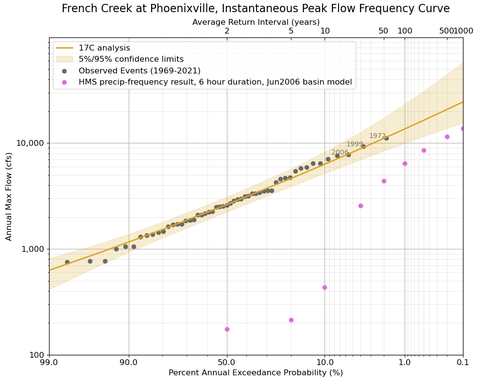
The reason for the mismatch could be a number of components previously shown in the bulleted list. At this point, it's time to dig into the model results. Did we pick too short of a storm duration, or were our basin parameters suspect? In this case, the loss rates are one of the most influential parameters. For the 2-year event, nearly all of the precipitation is being lost and absorbed into the initial deficit. We know that's not right. Let's try the other extreme: set the initial deficit to 0 inches, which assumes complete soil saturation before the storm comes. The results are below. Looks as though we've overshot the mark juuust a bit.
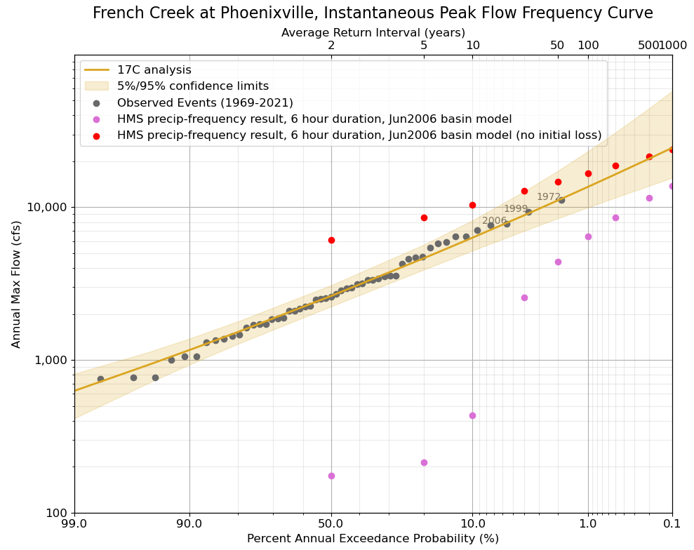
Now we are firmly in the territory of engineering judgment. It is clear that we shouldn't be assuming total saturation for a common event, like the 2-year, but that assumption probably is appropriate for an extreme event like the 1000-year. To be consistent with our physical understanding of the basin, we may consider defining initial losses as a function of event probability.
We must take care not to get tunnel vision and only focus on the initial loss parameter, when we know there are other parameters that also should be adjusted. And at the end of the day, we won't really have gained much if we spend a lot of effort just trying to match the flow-frequency curve from Bulletin 17C. If we do that, we'll basically end up with a series of precipitation-frequency runs that match the Bulletin 17C analysis, yielding little useful information. The goal is to have basin parameters that actually make physical sense at various frequencies, not just try to match a curve.
Let's turn our attention briefly to another key parameter–the unit hydrograph parameters (Tc and R). It is well established that as storm events get larger, the Tc and R parameters should decrease to represent a faster response as more runoff comes via overland flow. For instance, in many probable maximum flood (PMF) studies, the unit hydrograph parameters are "peaked" by 50% to represent this principle. Developing this relationship usually requires either calibration of large number of observed events of various magnitudes or using a 2-d simulation approach, as outlined in the tutorial here: Creating Variable Clark Transform Method Parameters using the 2D Diffusion Wave Transform Method. In our example, we haven't gone to the trouble of doing this. We'll assume the Tc and R parameter from the June 2006 calibration are appropriate for about the 10-year event, and the 50% peaked unit hydrograph parameters are appropriate for the 1000-year event. The estimates for the other events are interpolated.
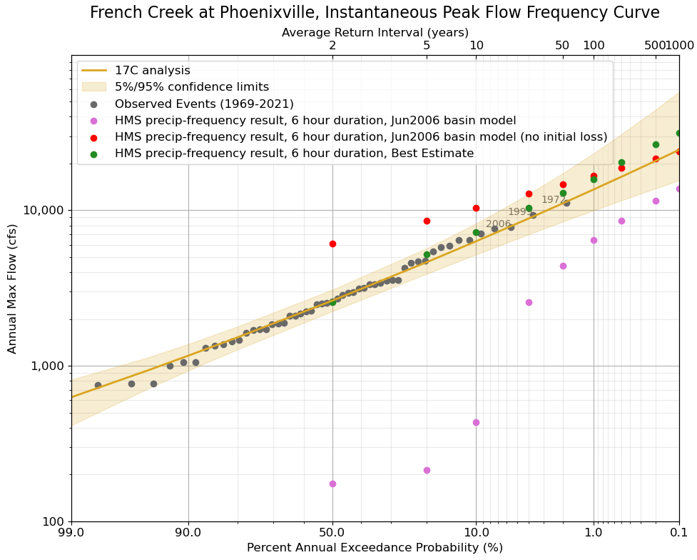
The adjustments to the basin model parameters are shown in the table below, with the results from the precipitation-frequency simulations in green.
| Event | Initial Deficit (inches) | Time of Concentration (hours), Storage coefficient (hours) |
|---|---|---|
| 50% (2-year) | 1.00 | 5.6 (Jan 1996 calibration) |
| 20% (5-year) | 1.00 | 5.1 |
| 10% (10-year) | 1.00 | 4.9 (Jun 2006 calibration) |
| 4% (25-year) | 1.00 | 4.5 |
| 2% (50-year) | 1.00 | 4.2 |
| 1% (100-year) | 1.00 | 4.0 |
| 0.5% (200-year) | 0.67 | 3.8 |
| 0.2% (500-year) | 0.28 | 3.5 |
| 0.1% (1000-year) | 0.00 | 3.3 (50% peaking) |
Uncertainty
There is a much better match now between the precipitation-frequency simulations and the Bulletin 17C curve. However, we shouldn't be too proud of ourselves, since we just manually tweaked two parameters to achieve a match in a way that seemed reasonable. There are many other components to the analysis that should be varied to capture the uncertainty from the precipitation-frequency estimates. A list of key components of uncertainty and possible approaches to uncertainty are given below:
- Precipitation amount: Confidence intervals from Atlas 14 may be used
- Storm duration: A slightly longer storm, like 12 hours, may be weighted equally with a 6 hour storm
- Temporal pattern of storm: Only one temporal pattern was used. Since the French Creek watershed is fairly small, the results will be very sensitive to the temporal distribution. Observed events or other NOAA Atlas 14 distributions may be used.
- Spatial pattern of storm: In larger watershed, this will be more important to vary. At French Creek, it is a relatively minor component.
- Antecedent conditions: Initial snowpack can be varied when applicable. At French Creek, we ignored rain-on-snow events . While the initial deficit was calibrated to the flow-frequency curve, there is still uncertainty in this parameter.
- Temperature sequence (for snowmelt contributions): Neglected for French Creek, but critical for snowmelt-driven systems.
- Basin loss rates and computational method. The constant loss rates can be varied.
- Basin unit hydrograph parameters and computational method. While unit hydrograph parameters were varied by event size, there is still uncertainty in this parameter.
- Basin baseflow parameters and computational method: When a recession baseflow model is used with a single storm event, it is not a sensitive parameter. If the linear reservoir approach is used, it becomes more important.
- Reservoir regulation effects (when applicable)
Ideally, all components would be varied in a Monte Carlo sampling framework. A key consideration when evaluating uncertainty in the results is whether the various components of uncertainty can be considered independent. Some parameters are likely independent, such as the uncertainty in precipitation-frequency amounts and the antecedent conditions. However, it is difficult to assume independence for uncertainty of all parameters. The opposite assumption from independence is perfect correlation, which is not appropriate either. If perfect correlation was assumed, the upper bound of a 90% confidence interval for peak flow would be estimated by performing a simulation with all parameters at the upper end of their 90% confidence interval. This combination of parameters is simply not plausible for upper uncertainty bound. Even so, runs using the perfect correlation assumption can be used a check on the uncertainty bounds from Bulletin 17C at extreme events. An example of doing this is shown below for the 1000-year event. For this simulation, the following assumptions were used:
- Precipitation amount: Upper bound of 90% interval from Atlas 14. Maintained areal reduction factors from TP-40.
- Storm duration: Did both a 6-hour storm and a 12-hour storm
- Temporal pattern of storm: Used more extreme temporal distribution from NOAA Atlas 14: 2Q 10%.
- Spatial pattern of storm: No change.
- Antecedent conditions: Initial deficit set to 0.
- Temperature sequence (for snowmelt contributions): Neglected for French Creek.
- Basin loss rates and computational method. Constant loss reduced from 0.09 to 0.06.
- Basin unit hydrograph parameters and computational method. Tc and R set to 3 hours.
- Basin baseflow parameters and computational method: No change.
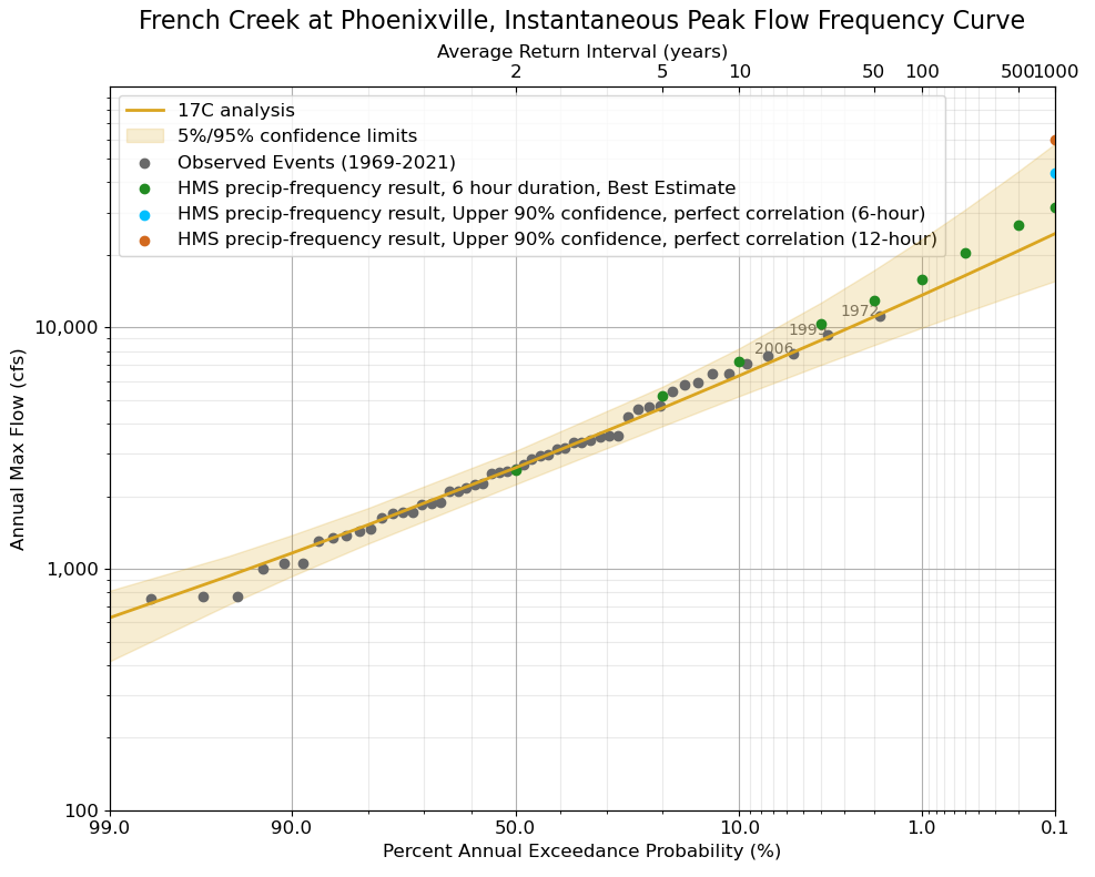
The 12-hour storm duration results in a significantly higher peak than the 6-hour storm, throwing a bit of cold water on our earlier assumption that 6-hour was best. However, even when all parameters are pushed their extremes simultaneously, the upper bound estimate from the precipitation-frequency simulation approach is lower than the Bulletin 17C bound. Provided we have confidence in the NOAA Atlas 14 precipitation-frequency curve uncertainty, this suggests the uncertainty bounds from Bulletin 17C may be a bit overstated for the extreme events.
Sometimes, the uncertainty introduced from the various components will be larger than the Bulletin 17C uncertainty bounds. In these cases, the value added from including the precipitation-frequency simulations is limited.
Combining the two approaches
Ultimately, it is up to the judgment of the analyst to decide if the precipitation-frequency simulation results are reliable enough to merit combining them with the Bulletin 17C result. A Bulletin 17C analysis is nearly always the best estimate for the more common range of event frequencies. A typical approach to incorporate precipitation-frequency simulation information to the flow-frequency curve is to "blend" the 17C analysis with the precipitation-frequency results. This "blending" process is akin to weighting the two approaches. For instance, the precip-frequency results might be used exclusively for events more rare than the 1000-year event, and the Bulletin 17C results might be used exclusively for events more common than the 10-year event. For the probabilities in-between, the estimates from the two approaches are weighted to effect a smooth transition. This approach is described within Appendix 9 of Bulletin 17C (England et al., 2019).
An example application that demonstrates how a Bulletin 17C flow-frequency curve can be combined with flow-frequency information from precipitation-runoff modeling using HEC-HMS can be found here.
If a Bayesian approach is being used to estimate flow-frequency, a range of HEC-HMS simulations for a given AEP event can be used as prior information. Applications like RMC-BestFit can be used to combine these two sources of information using Bayesian estimation techniques: https://www.rmc.usace.army.mil/Software/RMC-BestFit/.
Conclusion
This tutorial compared a basic Bulletin 17C analysis with an approach using precipitation-frequency curves in conjunction with an HEC-HMS model. The example was a very simple watershed, but even so, the process of incorporating precipitation-frequency information is certainly not straightforward or a cookbook process. There are multiple interdependent processes at play when estimating runoff from a precipitation volume that make calibration to existing flow-frequency information a critical step in the process. Even then, the calibration to flow-frequency information must stay within physically reasonable bounds. This example helped illustrate the high degree of uncertainty present if no flow data is available. If no flow data were available and only the precipitation-frequency information was used, the assumptions in the HEC-HMS model become even more difficult to defend, and the uncertainty bounds should be shown very generously.
The code used to produce the graphics can be found here: GraphsPython.zip.