HEC-HMS Setup
Introduction
The HMS model development process is set up to capture basin and meteorologic variability within the watershed. Variability arises from temporal changes—seasonal patterns of rainfall and snowmelt, storm-to-storm differences in intensity and duration and interannual wet-dry swings—as well as spatial heterogeneity in soils, land cover, topography and rainfall distribution. The HMS model can capture this variability by sampling from key basin parameters including transform, baseflow, and soil loss to produce a range of possible flow-frequency hydrographs instead of a single deterministic hydrograph. Representing variability allows for the uncertainty quantification needed for infrastructure design and provides greater transparency in model predictions for both common and rare events.
This section describes the HEC-HMS calibration process, storm specific-depth area reduction, and storm temporal patterns. The HMS model was calibrated to multiple storm events using gridded precipitation. The calibrated parameters are collected for use in the subsequent Monte Carlo analysis. The gridded precipitation dataset from the calibration was further used to create event-specific depth area reduction curves and temporal patterns for the Monte Carlo simulation. Additionally, a continuous simulation model was also developed and calibrated to create a distribution function of antecedent soil moisture and baseflow estimates.
HEC-HMS model development provides the following for the Flood Risk Analysis simulation:
- calibrated basin parameters
- precipitation-frequency duration assessment
- temporal patterns
- depth area reduction
- moisture deficit and baseflow cumulative distribution function.
HEC-HMS Configuration
The HEC-HMS model computes hydrographs that will be used to create empirical flow-frequency curves. HEC-HMS will also provide temporal patterns and depth area reduction functions that will be used for the Hydrologic Sampler Plugin. The HEC-HMS model was developed in version 4.12. This model was originally obtained from Modeling Flow-Frequency Relationships using HEC-HMS. The watershed area was delineated starting from the San Lorenzo River gage location using the delineation features in HEC-HMS. The watershed is represented as a single basin.

The basin processes used in the model are described in the table below.
| Process | Method |
|---|---|
| Loss | Deficit and Constant |
| Transform | Variable Clark Unit Hydrograph |
| Baseflow | Linear Reservoir Baseflow |
| Discretization | Structured |
| Meteorology | Gridded Precipitation |
The Gridded Precipitation method was selected as the Meteorological Model for model calibration.
1.Calibration
The calibration process is used to identify a set of parameters that reasonably reproduces the watershed hydrograph response for both peak flow and volume. The model was calibrated to 10 events using gridded rainfall from Multi-Radar Multi-sensor (MRMS) Quantitative Precipitation Estimates (https://mtarchive.geol.iastate.edu/) and Analysis of Period of Record Calibration (AORC - https://hydrology.nws.noaa.gov/pub/AORC/V1.1/). The more recent datasets used MRMS while the older storm events used AORC. The gridded data was normalized to daily Parameter-elevation Regressions on Independent Slopes Model (PRISM) grids.
The calibration process adjusted the following parameters:
- Transform parameters - time of concentration and storage coefficient used to match the peak flow timing and hydrograph shape.
- Loss parameters - initial deficit and constant rate used to match the hydrograph volume and peak flow value.
- Baseflow parameters - initial baseflow, baseflow coefficient, and baseflow fraction used to match the recession limb of the hydrograph and hydrograph volume.
These parameters had the greatest impact on the simulated hydrograph peak flow and volume. The calibrated parameters are then collected for use in the subsequent Monte Carlo analysis. Additionally, the selected storm events—events where the simulation demonstrated good agreement with observed flows during calibration—will be further analyzed to extract their temporal patterns and to develop storm-specific areal reduction curves.
| Storm Event | Gridded Data Source | RMSE | NSE | Percent Bias | R² | Performance Rating |
|---|---|---|---|---|---|---|
| Dec 29, 2022 - Jan 4, 2023 | MRMS | 0.2 | 0.952 | 7.28 | 0.96 | Very Good |
| Jan 6 - Jan 12, 2023 | AORC | 0.6 | 0.67 | 18.56 | 0.73 | Satisfactory |
| Jan 10 - Jan 17, Jan 2023 | MRMS | 1.0 | 0.082 | 23.42 | 0.60 | Unsatisfactory |
| Jan 14 - Jan 19, 2019 | MRMS | 0.3 | 0.881 | 2.74 | 0.91 | Very Good |
| Feb 5 - Feb 11, 2017 | MRMS | 0.1 | 0.981 | 1.46 | 0.98 | Very Good |
| Mar 3 - Mar 9, 2016 | MRMS | 0.2 | 0.961 | 6.25 | 0.96 | Very Good |
| Feb 1 - Feb 6, 1998 | AORC | 0.3 | 0.881 | 2.83 | 0.88 | Very Good |
| Mar 8 - Mar 13, 1995 | AORC | 1.6 | -1.592 | 4.40 | 0.07 | Unsatisfactory |
| Feb 14 - Feb 22, 1986 (daily) | AORC | 1.12 | -0.273 | -57.95 | 0.63 | Unsatisfactory |
| Jan 1 - Jan 9, 1982 (daily) | AORC | 0.49 | 0.764 | -2.53 | 0.88 | Very Good |
Performance ratings are based on the recommendations of Moriasi et al. (2007, 2015) for flow simulation accuracy. Simulations that performed poorly appeared to be in the gridded precipitation temporal pattern and rainfall volume distribution. Regardless of the rainfall-runoff modeling adjustments, the simulated hydrograph could not match the results reasonably. The parameter values for "Unsatisfactory" events were not included for further analysis, such as creating the Parameter Table (Transform, Loss, and Baseflow). The Parameter Table will be used to set up the Parameter Value Sample Table for sampling hydrologic variability or will be used to compute the best estimate value for a basin parameter.


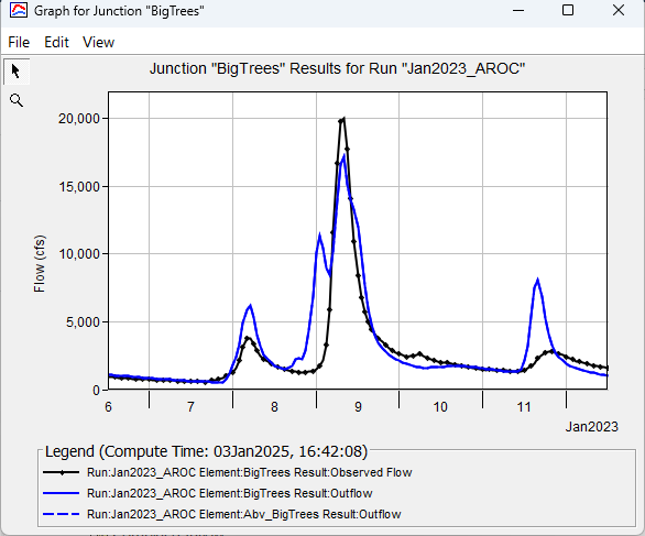
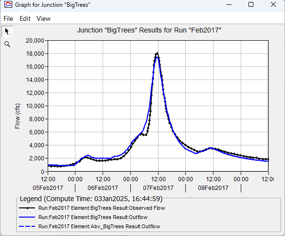
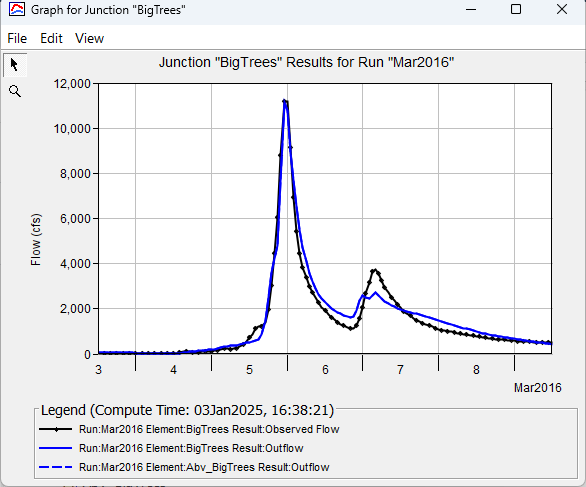
Graphical calibration results are shown for the parameters listed in the parameter table. Each plot displays time (days) on the x‑axis and discharge (cubic feet per second) on the y‑axis. The figures compare the simulated hydrograph (blue) from the calibrated HEC‑HMS model to the observed streamflow (black) at the gage location. In each case, the simulated hydrograph aligns closely with the observed hydrograph in terms of timing of the peak, magnitude of the peak flow, total runoff volume, and overall hydrograph shape, including the recession limb. Minor discrepancies occur during low‑flow periods, but overall agreement indicates that the calibrated parameters produce an accurate and physically consistent representation of watershed response.


Transform Parameter Table
| Event | Tc (hr) | R (hr) |
|---|---|---|
| Dec 29, 2022 - Jan 4, 2023 | 6 | 2.5 |
| Jan 6 - Jan 12, 2023 | 4 | 2.5 |
| Jan 14 - Jan 19, 2019 | 5 | 3.5 |
| Feb 5 - Feb 11, 2017 | 5.5 | 4 |
| Mar 3 - Mar 9, 2016 | 3 | 4 |
| Feb 1 - Feb 6, 1998 | 2 | 4 |
| Jan 1 - Jan 9, 1982 | 5 | 4 |
Loss Parameter Table
| Event | Initial Deficit (in) | Max Deficit (in) | Constant Rate (in/hr) | Impervious (%) |
|---|---|---|---|---|
| Dec 29, 2022 - Jan 4, 2023 | 1 | 8 | 0.22 | 0 |
| Jan 6 - Jan 12, 2023 | 1 | 8 | 0.12 | 0 |
| Jan 14 - Jan 19, 2019 | 0.1 | 8 | 0.15 | 0 |
| Feb 5 - Feb 11, 2017 | 0.8 | 8 | 0.15 | 0 |
| Mar 3 - Mar 9, 2016 | .08 | 8 | 0.22 | 0 |
| Feb 1 - Feb 6, 1998 | 1.2 | 8 | 0.15 | 0 |
| Jan 1 - Jan 9, 1982 | 0.5 | 8 | 0.12 | 0 |
Baseflow Parameter Table
| Event | Initial Baseflow (cfs/mi2) | GW1 Fraction | GW1 Coefficient (hr) | GW1 Reservoirs | Initial Baseflow 2 (cfs/mi2) | GW2 Fraction | GW2 Coefficient (hr) | GW2 Reservoir |
|---|---|---|---|---|---|---|---|---|
| Dec 29, 2022 - Jan 4, 2023 | 0.5 | 0.3 | 10 | 2 | 1 | 0.05 | 100 | 1 |
| Jan 6 - Jan 12, 2023 | 4 | 0.4 | 10 | 2 | 6 | 0.1 | 100 | 1 |
| Jan 14 - Jan 19, 2019 | 0.5 | 0.2 | 15 | 2 | 0.5 | 0.1 | 50 | 1 |
| Feb 5 - Feb 11, 2017 | 0.5 | 0.4 | 15 | 1 | 9 | 0.5 | 100 | 1 |
| Mar 3 - Mar 9, 2016 | 0.2 | 0.3 | 15 | 2 | 0.3 | 0.1 | 50 | 1 |
| Feb 1 - Feb 6, 1998 | 1 | 0.4 | 15 | 1 | 2.5 | 0.2 | 50 | 1 |
| Jan 1 - Jan 9, 1982 | 0 | 0.4 | 20 | 2 | 0.5 | 0.1 | 100 | 1 |
2. Storm Duration
Storm duration and depth is a parameter in frequency storm modeling, which involves characterizing the statistical properties of rainfall events for various return periods. Storm duration defines the length of time over which rainfall intensity and volume are accumulated and directly influences the temporal distribution of precipitation inputs used in hydrologic analyses. Accurate representation and selection of the storm duration is essential when generating hypothetical storms—inadequate consideration of storm duration can lead to underestimation of runoff volumes and flood risks.
HEC-HMS allows users to input any storm duration as long as the corresponding frequency-depth data—representing rainfall depths associated with specific return periods—is available. This frequency-depth information is commonly obtained from NOAA Atlas 14, which provides precipitation depths for durations ranging from as short as 5 minutes up to 60 days. To evaluate how storm duration affects watershed response, a durational analysis was performed using Monte Carlo simulations in HEC-HMS. This approach involved sampling various rainfall depths, patterns, and areal reduction factors for the 1% Annual Exceedance Probability event. Storm durations of 12, 24, 48, and 96 hours were selected to represent a range from relatively short to extended storm events. The results, visualized with box-and-whisker plots shown below, indicate that average peak flows are highest for the 48-hour storm duration, with a slight decrease observed at the 96-hour duration. Selecting shorter durations such as 12 or 24 hours risks underestimating the total runoff volume that contributes to peak flows. Although the 72-hour duration was not explicitly evaluated, it may yield peak flows similar to or slightly exceeding those from the 48-hour scenario; however, differences between these longer durations are relatively minor and have limited practical impact. These findings suggest that using a longer storm duration—reflecting typical rainfall event lengths—is generally more appropriate for estimating peak flows than basing duration on the basin time of concentration, which some methodologies propose as an alternative (Chow et al., 1988;). The basin time of concentration represents the time it takes for runoff generated at the most distant point in a watershed to reach the outlet, but it may underestimate runoff volume when used as storm duration for frequency analysis.

Storm Specific Depth Area Reduction Development
Depth area reduction functions (DARF) are used to adjust point rainfall estimates (precipitation frequency depths) to represent average rainfall over larger areas. Since frequency depths precipitation estimated at a single point are greater than the average over a broader area, DARFs provide scaling factors that reduce these point depths based on the size of the area of interest. In frequency flow modeling, these functions are essential for converting precipitation frequency data (e.g., 100-year, 24-hour rainfall at a point) into areal-average values appropriate for hydrologic models (usually the watershed area).
In practice, regionalized DARFs are used for hypothetical storm modeling, such as TP-40-49 and depth area functions in Hydrometeorological Report (HMR) documents. These curves are created from historic storms and generalized for a given region. For this analysis, rather than use a regionalized DARF, a unique DARF for each historic storm is created and treated as a variable parameter in the rainfall-runoff model. Storm specific depth–area reduction curves were developed for each event that yielded "Satisfactory" calibration results, as these storms exhibited temporal patterns and depths that could closely reproduce observed hydrograph. The reduction curves were created using MetVue 3.2 and described in Creating Depth-Area Reduction Curves from Gridded Precipitation Data. The storm depth area reduction curves were created for the 48 hours duration for areas out to 200 square miles, shown in the Table and Figure below. The reduction factors were applied for the watershed area of 106 square miles and will be put into the Scripting Plugin to reduce the precipitation-frequency rainfall depths.
| Area (sq mi) | 2017 | 2019 | 1982 | 2016 | 2023-1st | 2023-3rd | 1998 | 2023-2nd | HMS 59 |
| 10 | 1.00 | 1.00 | 1.00 | 1.00 | 1.00 | 1.00 | 1.00 | 1.00 | 1.00 |
| 20 | 0.99 | 0.98 | 0.97 | 0.98 | 0.99 | 0.99 | 0.97 | 0.99 | |
| 30 | 0.97 | 0.95 | 0.95 | 0.97 | 0.98 | 0.98 | 0.93 | 0.98 | |
| 40 | 0.96 | 0.93 | 0.92 | 0.96 | 0.97 | 0.97 | 0.90 | 0.97 | |
| 50 | 0.94 | 0.90 | 0.89 | 0.95 | 0.96 | 0.95 | 0.88 | 0.96 | 0.92 |
| 60 | 0.93 | 0.88 | 0.86 | 0.94 | 0.95 | 0.94 | 0.87 | 0.95 | |
| 70 | 0.92 | 0.85 | 0.85 | 0.93 | 0.94 | 0.93 | 0.86 | 0.94 | |
| 80 | 0.90 | 0.84 | 0.84 | 0.92 | 0.94 | 0.92 | 0.86 | 0.93 | |
| 90 | 0.89 | 0.82 | 0.83 | 0.91 | 0.93 | 0.91 | 0.85 | 0.92 | |
| 100 | 0.87 | 0.81 | 0.82 | 0.90 | 0.92 | 0.90 | 0.84 | 0.92 | 0.89 |
| 106 | 0.86 | 0.80 | 0.81 | 0.89 | 0.91 | 0.89 | 0.83 | 0.91 | 0.88 |
| 200 | 0.73 | 0.70 | 0.73 | 0.82 | 0.85 | 0.82 | 0.77 | 0.84 | 0.85 |

TP-40-49 and HMR-59 Depth Area Reduction Curves are plotted alongside the storm specific Depth Area Curves. TP-40-49 is consistently has a higher ratio thus a lower reduction compared to the storm specific reduction while HMR-59 falls close to the storm specific curves. TP-40-49 is a national reduction curve and was developed with relatively few storms. It is highly encouraged to choose a region specific reduction curve (i.e. HMR-59) or develop one for your specific region.
3. Storm Specific Temporal Patterns
Rainfall temporal patterns describe how rainfall intensity varies over the duration of a storm event, strongly influencing both the timing and magnitude of runoff response in frequency storm modeling. The distribution of rainfall within a storm determines when peak flows occur and how much water reaches the outlet, affecting the shape and height of the hydrograph. In practice, standardized temporal patterns—such as the classic pyramid-shaped hyetograph or those derived from regional analysis (e.g., NRCS Type II or NOAA Atlas 14)—are commonly applied to represent storm events. Additionally, precipitation-frequency depths are “nested,” meaning that shorter-duration depths (e.g., 1-hour) are contained within longer durations (e.g., 3-hour), which can result in conservative design hydrographs and sometimes unrealistic storm profiles for extended durations.
The timing of peak rainfall within these patterns is often critical; placing the heaviest rainfall near the beginning, middle, or end of a storm can significantly alter peak flow predictions. Instead of relying on a standardized or single historical pattern, this analysis considered temporal patterns as variable parameters. For this purpose, historical storm patterns that demonstrated at least satisfactory calibration were selected and treated as variable inputs. Temporal patterns were generated for each historical storm over 48-hour durations, as illustrated in the figure below. These patterns include front-loaded, middle-loaded, and back-loaded storm types. They are stored in HEC-DSS under the "Precip-Inc" Part-C pathname and will serve as inputs for the Hydrologic Sampler Plugin.

4. Continuous HEC-HMS Simulation Model
Continuous simulation modeling in hydrologic models involves the long-term representation of watershed processes to realistically capture the dynamic interactions among key components such as evapotranspiration (ET), soil moisture, and baseflow. Unlike event-based models that focus on individual storms, continuous simulation tracks the evolving state of the hydrologic system over extended periods. By incorporating ET, the model accounts for water loss to the atmosphere through plant transpiration and soil evaporation, which influences soil moisture levels. Soil moisture dynamics are important for controlling infiltration, runoff generation, and groundwater recharge, while baseflow represents the sustained contribution of groundwater to streamflow during dry periods.
The primary objective of the continuous simulation model is to generate a probability distribution of initial soil moisture and baseflow states preceding storm events. Initial soil moisture, often referred to as antecedent moisture, represents the condition of soil water content immediately before a significant rainfall event. Numerous studies have demonstrated that initial soil moisture is among the most sensitive parameters affecting peak flow, total runoff volume, and hydrograph shape when compared to other model inputs and parameters (e.g., precipitation characteristics, model structure). For example, Newman et al. (2021) found that within their watershed modeling framework, initial conditions showed greater influence on flow outputs than both model parameters and precipitation inputs. Their analysis showed the selection of antecedent moisture had a large influence in hydrologic prediction. Similarly, Ahmadisharaf et al. (2018) highlighted antecedent moisture content (AMC) as a key driver controlling not only peak discharge but also the duration and volume of runoff events. Their findings point out initial moisture states can have a large effect on the predictions of flood magnitude and timing and should be considered carefully.
In HEC-HMS, the Initial Deficit parameter represents the initial moisture state and the rainfall volume must satisfy the deficit prior to runoff generation. A moisture deficit time series and baseflow time series will be extracted and a probability distribution created from the moisture deficit and baseflow time series.
HEC-HMS has continuous simulation capabilities with the ability to incorporate Evapotranspiration and soil moisture wetting and drying (Deficit and Constant Loss method) and volume accounting (Linear Reservoir Baseflow) for sustained baseflow. The event-based San Lorenzo model was used as the starting point which already had Deficit and Constant and Linear Reservoir baseflow as methods selected. The Hamon method was selected to represent ET in the Meteorological Model and the Simple Surface method was added to the Basin Model. The Meteorological Model was set up using the Specified Hyetograph method. The transform method was switched to using the Variable Clark method. This method allows the Tc and R parameters to increase or decrease as a function of rainfall intensity and requires a Paired Data Type - Percentage Curve to describe the rainfall intensity to transform relationship. A tutorial on creating the Paired Data Percentage Curve is described here.
Precipitation and Temperature data was downloaded from the AORC gridded dataset for 1979 - 2024. Once downloaded, the grids were clipped to the watershed domain and converted from a gridded timeseries to a basin average time-series using the Grid to Point tool in HEC-HMS. Converting from a gridded compute to a basin average time-series speeds up the compute time with negligible differences in the outputs for this watershed basin.
As of 2024, the following python script (Python 3.10) was used to download the AORC data. These files will be downloaded in 1 hour increments. The total file size will be > 60 GB for both temperature and precipitation grids.
The continuous simulation calibration process followed a similar process outlined in this tutorial. After linking rainfall inputs to the model, basin model parameters were initially set based on the average values from event-based model calibrations.
| Hamon Coefficient | Crop Coefficient | Constant Loss | Max Deficit | Time of Concentration (hr) | Storage Coefficient (hr) | GW1 Fraction | GW1 Coefficient | GW2 Faction | GW2 Coefficient | GW3 Fraction | GW3 Coefficient | |
|---|---|---|---|---|---|---|---|---|---|---|---|---|
| Initial | 0.0065 | 1 | 0.16 | 8 | 4.2 | 3.7 | 0.3 | 14 | 0.2 | 80 | - | - |
| Calibrated | 0.0085 | 1 | 0.25 | 8 | 4 | 6 | 0.3 | 50 | 0.2 | 500 | 0.2 | 3000 |
During summer months, when rainfall is minimal along the San Lorenzo watershed, streamflow is primarily sustained by baseflow. To better capture this behavior, an extra baseflow layer was added and baseflow coefficients were increased, which effectively delayed flow routing and allowed the model to simulate sustained baseflow during dry periods.
The calibration aimed to achieve at least a Satisfactory performance rating. Adjustments to the constant loss parameter improved volume simulations, as indicated by Pbias, while increasing the storage coefficient improved NSE and R². The Calibration App, described in the tutorial, was used to compare daily simulated and observed time series and provided the NSE, RSR, R², and Pbias metrics. Simulated outputs were also visually compared against a peak flow-frequency curve. Initially, simulated peak flows tended to exceed those observed at common recurrence intervals. Refining the storage coefficient percentage curve improved the frequency curve alignment with observed data. The final calibrated parameters, performance metrics, and frequency curve comparisons are presented below.


Once the continuous simulation model was calibrated, the moisture deficit and baseflow hourly time-series were extracted from the model and used to create durational curves. This can be done using HEC-SSP or the Math Function tool in HEC-DSS. The duration curve represents the percentage of time that a specific moisture deficit or baseflow value is equaled or exceeded. In other words, it plots exceedance probability against moisture deficit or baseflow magnitude. Monthly durational curves were generated and incorporated into the HEC-HMS model as Paired Data Type Cumulative Distribution Functions (CDFs). To convert the duration curves into CDFs, their complements were taken by calculating 1− (duration curve).


5. HEC-HMS model for WAT
The HEC-HMS model was configured for use with the HEC-WAT Flood Risk Analysis compute. A new HMS model was created based on the Basin Model setup from the continuous simulation. The Meteorological Model was configured to use a Specified Hyetograph, and an Uncertainty Analysis compute type was created. As described in the continuous simulation calibration, Paired Data Cumulative Distribution Functions (CDFs) were added for soil moisture deficit and baseflow.
The Baseflow Initial Type originally used Discharge Per Area for the event and continuous based models. This option was changed to Discharge for the WAT model since the Cumulative Distribution Function will select a Discharge value to initialize the baseflow.
Additionally, Paired Data Parameter Value Samples were generated for Baseflow Coefficients 1 and 2, Baseflow Fractions 1 and 2, Constant Loss, Storage Coefficient, and Time of Concentration, all derived from the Parameter Tables. The parameters were organized such that each index corresponds consistently to a specific calibration event—for example, all parameter values related to the January 2019 event share the same index. This structured ordering will allows parameter sets to remain consistent with their respective calibration events.
The Parameter Table from the event model calibration and the CDF functions from the Continuous Simulation is added to the Uncertainty Analysis compute by adding Parameters to the compute type. During the Flood Risk Analysis compute, HEC-WAT will select a parameter from the Parameter Value Sample which is used for the basin model parameter. The Initial Deficit and Initial Baseflow will be selected based off the CDF function.
HEC-HMS Models for Download
Calibration Model: SanLorenzo_Calibration.zip
Period of Record Model: SanLorenzo_POR.zip
HEC-WAT HMS model: SanLorenzo_WAT.zip