Download PDF
Download page Modeling Flow-Frequency Relationships using HEC-HMS.
Modeling Flow-Frequency Relationships using HEC-HMS
Overview
In this workshop you will become familiar with the HEC-HMS software and available modeling options that can assist you in estimating a flow-frequency curve using precipitation-frequency information, characteristics of storm events, and a hydrologic model. Flow-frequency information computed by an HEC-HMS model will be compared to flow-frequency information computed following Bulletin 17C procedures within the HEC-SSP software.
Download a copy of all files for the following tasks - tutorial-files.zip
Introduction
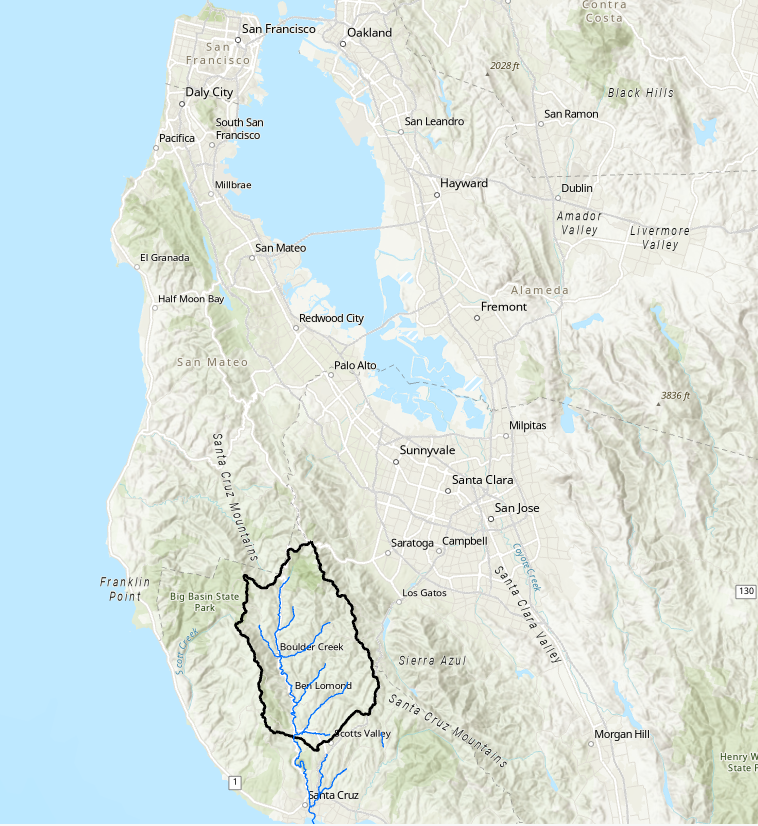
A portion of the San Lorenzo River watershed will be used for this workshop, the area above the San Lorenzo River at Big Trees CA streamflow gage (USGS gage 11160500). As shown below, the San Lorenzo River is located in Northern California, west of San Jose. The San Lorenzo River flows through Santa Cruz before it empties into Monterey Bay and the Pacific Ocean. The watershed is in the Santa Cruz Mountains, the land use type is mostly forested. The drainage area is 106 square miles.
Tasks in this workshop include:
- Task 1: Use HEC-SSP and Perform a Bulletin 17C Analysis
- Task 2: Become Familiar with the Calibrated HEC-HMS Models of the Study Watershed
- Task 3: Add Model Components for Hypothetical Storms
- Task 4: Configure and Run a Frequency Analysis Simulation
- Task 5: Analyze Results and Make Model Adjustments
- Task 6: Explore Impacts to Flow-Frequency with a Different Time Patterns
Task 1: Use HEC-SSP and Perform a Bulletin 17C Analysis
In this task you will create a new HEC-SSP project, import peak flow data for the San Lorenzo River at Big Trees CA streamflow gage, and perform a Bulletin 17 analysis.
- Download the Peak Flow data contained in the following HEC-DSS file to your computer - SanLorenzoRiver_atBigTreesCA_PeakFlow.dss.
- Create a new HEC-SSP project, name the project SanLorenzoRiver_atBigTreesCa.
- Use the data import wizard and import the peak flow data in this SanLorenzoRiver_atBigTreesCa_PeakFlow.dss file.
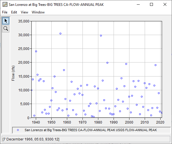
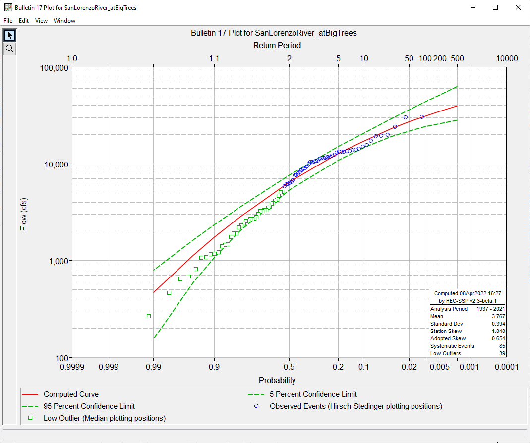
- The following figure shows the peak flow values, there are 85 annual maximum peak flow values, from 1937 through 2021.
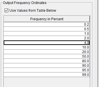
- Create a new Bulletin 17 analysis, name the analysis SanLorenzoRiver_atBigTrees. Select the peak flow dataset. Then edit the Output Frequency Ordinates table and change the 5 Percent Frequency Ordinate to 4 Percent (25-year return period).
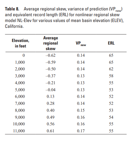
A regional flow frequency study was performed for the state of California in 2006. You can access this report from https://pubs.usgs.gov/sir/2010/5260/pdf/sir20105260.pdf. The regional skew study found a significant relationship between the average watershed elevation and the regional skew estimate. The figure below shows Table 8 in the report. The average elevation for the watershed upstream of the San Lorenzo River at Big Trees CA gage is 365 feet. Within the Bulletin 17 analysis, check the radio button to Use Weighted Skew. Then enter a Regional Skew of -0.61 and a Reg. Skew MSE of 0.14.

Reference
Parrett, C., Veilleux, A., Stedinger, J.R., Barth, N.A., Knifong, D.L., and Ferris, J.C., 2011, Regional skew for California, and flood frequency for selected sites in the Sacramento–San Joaquin River Basin, based on data through water year 2006: U.S. Geological Survey Scientific Investigations Report 2010–5260, 94 p.
- Compute the flow frequency curve. The figure below shows the plot and LPIII distribution parameters. Notice the Multiple Grubbs Beck test identified 39 low outliers.
Task 2: Become Familiar with the Calibrated HEC-HMS Models of the Study Watershed
The Initial HEC-HMS project files can be downloaded here - SanLorenzo_initial.zip. Open this project with HEC-HMS version 4.10 or newer. The model domain is represented with one subbasin element. Gridded precipitation from the Analysis of Period of Record for Calibration (AORC) dataset was used for the January 1982 calibration event. Gridded precipitation from the Multi-Radar Multi-Sensor Quantitative Precipitation Estimate (MRMS) dataset was used for the February 2017 and January 2019 calibration events.
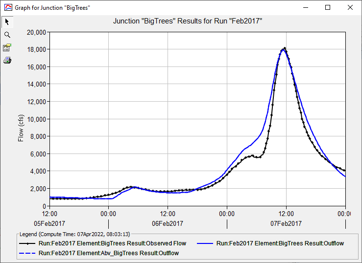
- Open the Feb2017 basin model, select the Feb2017 simulation run, run the simulation and view results at the BigTrees junction element. Results should look like the figure shown below. Results from the HEC-HMS model are the blue line and the observed flow is the black line. The model metrics show the Nash-Sutcliff is 0.96 and the percent error in runoff volume is 8.07%. The model is able to accurately simulate the precipitation-runoff response for this watershed and event.
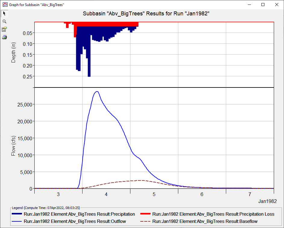
- Examine the other two basin models and simulation results, Jan1982 and Jan2019. Plot results for the subbasin element to see the precipitation hyetographs for these historical events. The figure below shows the subbasin plot for the Jan1982 event. Notice how the Jan1982 event exhibited intense precipitation at the beginning of the storm. We would refer to this as a front loaded storm. When you take a look at the Hyetograph for the Feb2017 event you will notice this event is more back loaded, the intense precipitation occurred a the end of the storm.
An effort was made when calibrating the basin model to use consistent parameters, when possible, and to ensure parameters stayed within reasonable ranges. The table below contains pertinent model parameters from the three calibration events.
The initial loss and initial baseflow values were adjusted to match initial soil moisture and channel flow conditions at the beginning of the simulation time window (initial conditions are based on the state of the watershed at the beginning of the simulation).
The GW 1 Coefficient was purposely set equal to the Clark Storage Coefficient. However, the number of GW 1 Reservoirs was increased to 3 to account for the lag and attenuation experienced by precipitation that infiltrates into the soil and then flows back onto the land surface due to interflow processes.Event Initial Loss
(in)
Constant Loss Rate
(in/hr)
Time of Concentration
(hr)
Storage Coefficient
(hr)
GW 1 Initial Flow
(cfs/sqmi)
GW 1
Fraction
GW 1
Coefficient
GW 1
Reservoirs
GW 2 Initial Flow
(cfs/sqmi)
GW 2
Fraction
GW 2
Coefficient
GW 2
Reservoirs
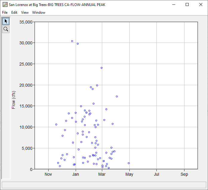
Feb2017 0.9 0.09 5 5 0.5 0.4 5 3 9.0 0.1 50 1 Jan1982 0.5 0.08 4 5 0.0 0.4 5 3 0.5 0.1 50 1 Jan2019 0.5 0.12 4 5 5.0 0.4 5 3 7.0 0.1 50 1 - The following figure shows the Year-over-Year Plot for the annual maximum peak flows at the San Lorenzo River at Big Trees CA gage. Notice how peak flows occur between November and April. The San Lorenzo watershed can experience months without precipitation between May and November. A significant amount of precipitation can be lost due to dry soil conditions in November and December after extended periods of little to no precipitation. Initial soil conditions are generally saturated between late December and the end of February, initial losses would be smaller for events occurring during these months. Initial soil conditions are generally dryer for events occurring in November/early December and after March 1. Because of these variable initial conditions, two different basin models were created for the hypothetical storm simulations. The CalibratedModel_dry and CalibratedModel_wet basin models were already added to the project for you. The CalibratedModel_dry basin model will be used for hypothetical floods that fall on drier watershed conditions and the CalibratedModel_wet basin model will be used for hypothetical floods that fall on wetter watershed conditions.
The variable Clark option in HEC-HMS allows you to create a relationship between excess precipitation and the time of concentration and storage coefficient parameters. For this model application, large flood events were used to estimate the time of concentration and storage coefficient values, but some of the hypothetical floods we are simulating in this workshop have much higher precipitation rates than the historical events used during model calibration. The reason why this modeling capability is important is because the precipitation-runoff response in a watershed is non-linear. Water velocities and channel storage change as the depth of water increases. Using a static unit hydrograph to transform precipitation to runoff does not capture the non-linear change to to the runoff response as precipitation intensities increase.
The following figure shows the Transform tab for the Abv_BigTrees subbasin element - in the CalibratedModel_dry basin model. The calibrated time of concentration and storage coefficient values have been entered. The Variable Parameter option also requires an index excess precipitation rate and percentage curves. An index excess precipitation rate of 0.5 inches/hour was defined. This value was approximately the peak excess precipitation rate from the Feb2017 simulation. The time of concentration and storage coefficient percentage curves were developed following the procedure outlined in the following tutorial, https://www.hec.usace.army.mil/confluence/hmsdocs/hmsguides/applying-transform-methods-in-hec-hms/using-2d-flow-within-hec-hms/creating-variable-clark-transform-method-parameters-using-the-2d-diffusion-wave-transform-method.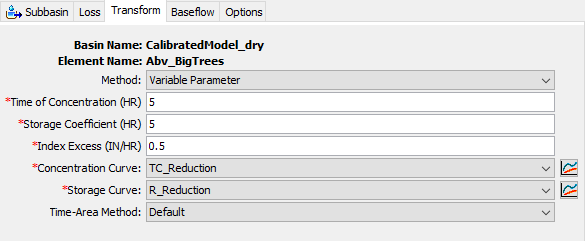
The following tables show the percent of reference excess precipitation vs percent of time of concentration and percent of storage coefficient. Using the following percentage curves and the default time of concentration, 5 hr, and storage coefficient, 5 hr, values with an index excess rate of 0.5 in/hr means the time of concentration would be reduced to 4.25 hours (0.85*5) and the storage coefficient will be reduced to 4.5 hours (0.9*5) if the excess precipitation rate was 1.0 inch/hour. You should notice the TC_Reduction and R_Reduction percentage curves have already been added to the project.Percent of Reference Excess Precipitation Percent of Time of Concentration Percent of Storage Coefficient 0 100 100 100 100 100 200 85 90 400 75 85 600 67 80 800 62 75 1000 60 75 The following table summarizes the model parameters defined in the calibrated basin models. Notice the initial loss and initial baseflow values are slightly adjusted for both wet and dry initial conditions.
Basin Model Initial Loss
(in)
Constant Loss Rate
(in/hr)
Time of Concentration
(hr)
Storage Coefficient
(hr)
GW 1 Initial Flow
(cfs/sqmi)
GW 1
Fraction
GW 1
Coefficient
GW 1
Reservoirs
GW 2 Initial Flow
(cfs/sqmi)
GW 2
Fraction
GW 2
Coefficient
GW 2
Reservoirs
CalibratedModel_dry 1.25 0.15 5 5 0.0 0.4 5 3 0.5 0.1 50 1 CalibratedModel_wet 0.25 0.1 5 5 0.5 0.4 5 3 9.0 0.1 50 1
Task 3: Add Model Components for Hypothetical Storms
In this task you will add multiple hypothetical storms to the HEC-HMS project that represent 50 percent through 0.2 percent storm events.
- Select the Components | Meteorologic Model Manager menu option. Within the Meteorologic Model Manager, click the New button to create a new meteorologic model and name it 0.2%_24hr_1982Pattern.
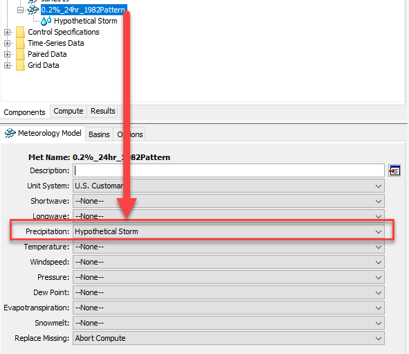
- Select the 0.2%_24hr_1982Pattern meteorologic model in the Watershed Explorer to open the Component Editor. Change the Precipitation Method to Hypothetical Storm as shown below.
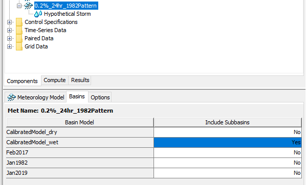
- Go to the Basins tab and set the Include Subbasins option to Yes for the CalibratedModel_wet basin model. In this workshop, only the 50% event will use the CalibratedModel_dry basin model. All other hypothetical storms will use the CalibratedModel_wet basin model.
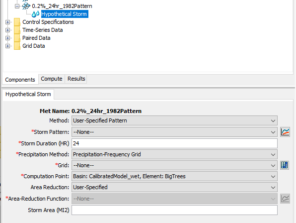
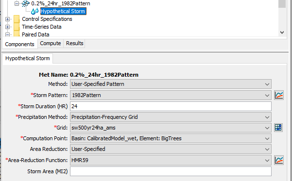
- Select the Hypothetical Storm node in the Watershed Explorer to open the Component Editor. As shown in the figure below, change the temporal pattern Method to User-Specified Pattern, enter a Storm Duration of 24 hours, select the Precipitation-Frequency Grid Precipitation Method, choose the BigTrees junction as the Computation Point, and set the Area Reduction option to User-Specified. More discussion about these choices is contained below.
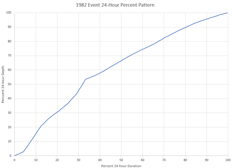
- The User-Specified Pattern option allows you to use your own normalized cumulative temporal pattern. The temporal pattern is defined as a percentage curve where the independent variable is percentage of the total storm duration. The dependent variable is percentage of the total storm depth. As the name of this meteorologic model implies, we are going to use the temporal pattern from the 1982 event. Open the following spreadsheet to see how a cumulative percent pattern was created for the maximum 24 hour window of the 1982 basin average hyetograph - HistoricPatterns.xlsx. The following figure shows the cumulative percentage pattern as contained in the spreadsheet.
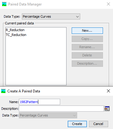
- To add a percentage pattern to HEC-HMS, select the Components | Paired Data Manager menu option to open the Paired Data Manager. Then within the Paired Data Manager, choose the Percentage Curve Data Type and click the New button. Enter a Name of 1982Pattern and then click the Create button to add the curve to the project.
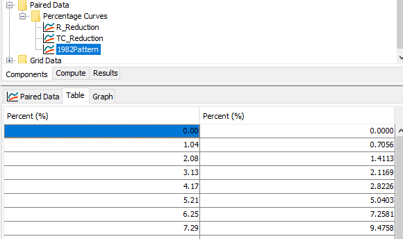
- Find the new 1982Pattern in the Paired Data folder in the Watershed Explorer. Open the Component Editor. The Data Source should be set to Manual Entry. Go to the Table tab and copy/paste the percent duration and percent total storm depth values from the spreadsheet contained in step 5. Your Table tab should look like the figure below. You can see a plot of the percentage curve on the Graph tab.
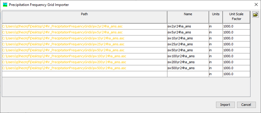
- Annual maximum 24-hour precipitation-frequency grids were downloaded from the NOAA Atlas 14 website, https://hdsc.nws.noaa.gov/hdsc/pfds/pfds_gis.html. Download and unzip the following zip file to your computer - 24hr_PrecipitationFrequencyGrids.zip. The zip file contains the 50% (2-yr), 20% (5-yr), 10% (10-yr), 4% (25-yr), 2% (50-yr), 1% (100-yr), 0.5% (200-yr). and 0.2% (500-yr) 24-hour precipitation-frequency grids for California.
- HEC-HMS contains a tool for importing precipitation-frequency grids. Select the File | Import | Gridded Data | Precipitation Frequency menu option. Within the Precipitation Frequency Grid Importer, select each of the precipitation-frequency grids downloaded in step 8. You can accept the default name or modify the name. Leave the Units as in (inches) and the Unit Scale Factor should be 1000.0. Click the Import button. You should notice in the pop-up message that the program created a copy of the grids and saved the copy to the project's data folder. You can find these grids in the Watershed Explorer, in the Grid Data | Precipitation Frequency Grids folder.
The next step is to add area-reduction information to the project. The hypothetical storm has two options for area-reduction, either the TP40 area-reduction curves or user-specified area-reduction curves. For this workshop, we are going to use area reduction information found in Hydrometeorological Report 59. The following table contains the area-reduction information for the California mid-coastal region.
Storm Area Area-Reduction Factor 10 1 50 0.91 100 0.87 200 0.825 500 0.76 1000 0.705 2000 0.64 5000 0.52 10000 0.42
Reference
P. Corrigan, D.D. Fenn, D. R. Kluck, and J.L. Vogel, 1999, Probable Maximum Precipitation for California: Hydrometeorological Design Studies Center, Office of Hydrology National Weather Service.
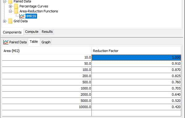
- Open the Paired Data Manager again and choose the Area-Reduction Functions Data Type. Click the New button and name the area-reduction curve HMR59. Find the new area-reduction curve in the Watershed Explorer and open the Table tab in the Component Editor. Manually enter the area-reduction information shown in step 10. The completed table should be similar to the figure shown below. Since the drainage area at the San Lorenzo River at Big Trees CA gage is 106.6 square miles, the Atlas 14 precipitation depths will be reduced by a factor slightly less than 0.87.
- Finally, all information has been added to the HEC-HMS project to complete the 0.2%_24hr_1982Pattern meteorologic model. Open the Hypothetical Storm Component Editor and choose the 1982Pattern Storm Pattern, the 0.2% (500-yr) precipitation frequency Grid, and the HMR59 Area-Reduction Function. The completed component editor should like the figure shown below.
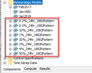
- Create 7 copies of the 0.2%_24hr_1982Pattern meteorologic model. Use the event's probability in each name, there should be Meteorologic Models for the 0.2%, 0.5%, 1%, 2%, 4%, 10%, 20%, and 50% events. After you create the additional meteorologic models, make sure the correct precipitation-frequency grid is selected in each one. The following figure shows the 8 hypothetical storm meteorologic models in the project.
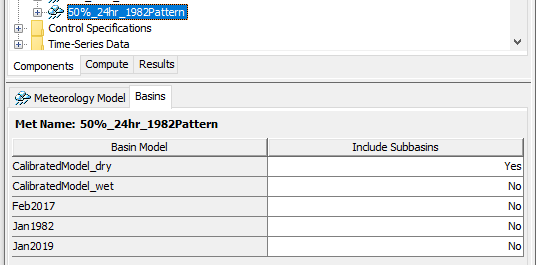
- The final step in this task is to make sure the 50%_24hr_1982Pattern meteorologic model is set up to work with the CalibratedModel_dry basin model. As shown below, open the Component Editor for the 50%_24hr_1982Pattern meteorologic model and then open the Basins tab. Change the Include Subbasins option from No to Yes for the CalibratedModel_dry basin model. Then change the Include Subbasins option from Yes to No for the CalibratedModel_wet basin model as shown below.
Task 4: Configure and Run a Frequency Analysis Simulation
The new Frequency Analysis compute type was added to HEC-HMS 4.10. The Frequency Analysis allows modelers to quickly run multiple meteorologic and basin model combinations where the meteorologic models represents an array of frequency based events.
- Select the Compute | Frequency Analysis Compute menu option to open the Create Frequency Analysis Wizard.
- Enter a name of Jan1982_TimePattern, click the Next button, and then click the Finish button.
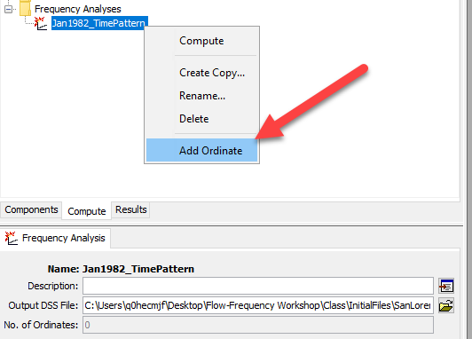
- Go to the Compute tab in the Watershed Explorer and expand the Frequency Analysis folder to see the Jan1982_TimePattern Frequency Analysis. As shown below, right click on top of the Frequency Analysis name and choose the Add Ordinate menu option. Think of the ordinate as a frequency based event, like the 0.2% event.
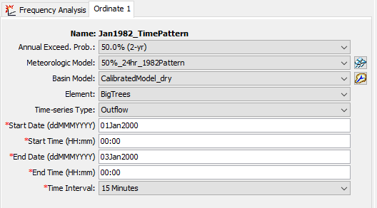
- Select the Ordinate 1 node in the tree to open the Component Editor. Organize your events so that ordinate 1 is the 50% event and ordinate 8 is the 0.2% event. As shown in the figure below, you want to match the meteorologic model with the Annual Exceedance Probability chosen for the event. The CalibratedModel_dry basin will be used for the 50% Annual Exceedance Probability event only, make sure you choose the CalibratedModel_wet basin model for all other ordinates. The Element is the location in the basin model where we want the frequency curve computed. The program uses this element location to compute the drainage area / storm area which is used by the Hypothetical Storm. Choose the Outflow Time-series Type. Enter a Start Date of 01Jan2000 and an End Date of 03Jan2000. Use 00:00 for both the start time and end time. The Time Interval should be set to 15 Minutes.
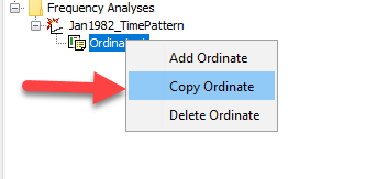
- Once you have Ordinate 1 filled out, you can copy the ordinate as shown below. Create a total of 8 ordinates.
The following table contains the Annual Exceedance Probability, Meteorologic Model, and Basin Model for each of the 8 ordinates. Make sure you correctly configure each of the ordinate Component Editors.
Annual Exceedance Probability Meteorologic Model Basin Model 50.0 % 50%_24hr_1982Pattern CalibratedModel_dry 20.0 % 20%_24hr_1982Pattern CalibratedModel_wet 10.0 % 10%_24hr_1982Pattern CalibratedModel_wet 4.0 % 4%_24hr_1982Pattern CalibratedModel_wet 2.0 % 2%_24hr_1982Pattern CalibratedModel_wet 1.0 % 1%_24hr_1982Pattern CalibratedModel_wet 0.5 % 0.5%_24hr_1982Pattern CalibratedModel_wet 0.2 % 0.2%_24hr_1982Pattern CalibratedModel_wet - Compute the Jan1982_TimePatern Frequency Analysis. You should see two progress bars, one tracks the overall compute and the other tracks the compute of each ordinate.
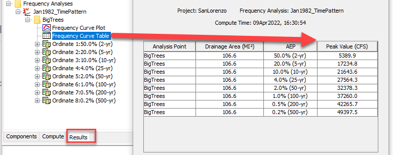
- After the compute finishes, go to the Results tab of the Watershed Explorer and expand the result tree for the BigTrees element as shown below. The Frequency Curve Plot shows the peak flow values in a probability plot and the Frequency Curve Table contains the peak flow values for each ordinate (event) as shown below.
Task 5: Analyze Results and Make Model Adjustments
Use the following spreadsheet to plot results from the HEC-HMS model simulations and compare results to the flow-frequency curve computed by the Bulletin 17 analysis in HEC-SSP - FlowFrequencyPlot_HMR59.xlsx. The Data tab contains the peak flows from the San Lorenzo River at Big Trees CA streamflow gage and the plotting position, computed flow-frequency curve, and confidence limits computed by the Bulletin 17 analysis in the HEC-SSP project created in Task 1. In this task, you will enter the results from the HEC-HMS Frequency Analysis into the yellow cells in Column M on the Data tab. Column N is configured to accept results from an additional HEC-HMS Frequency Analysis where a different 24-hour time pattern will be used. The spreadsheet's Plot tab is shown in the figure below. After you paste results from the HEC-HMS model, you can view how the precipitation-runoff modeling results compare to the Bulletin 17 analysis.
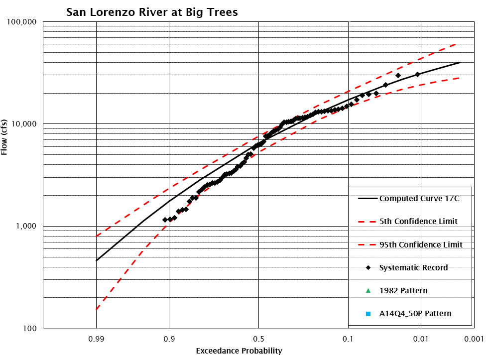
- Copy and Paste the peak flows from the Frequency Analysis computed in Task 4 into Column N, Data tab, in the FlowFrequencyPlot_HMR59.xlsx spreadsheet. Go to the Plot tab, your results should be similar to the figure shown below.

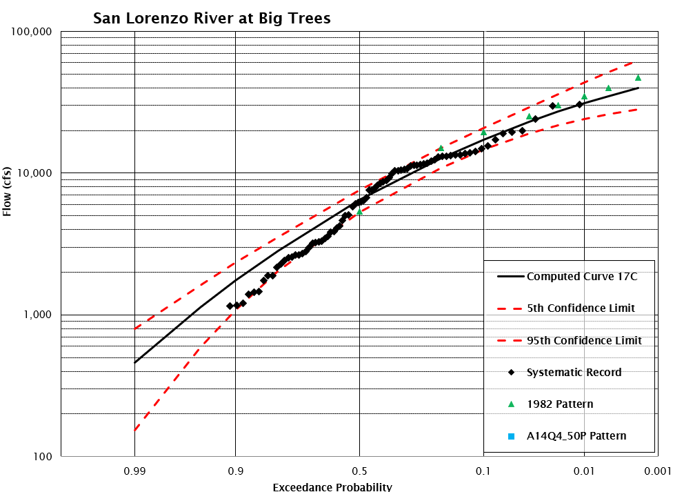
- Forcing flow-frequency results from precipitation-runoff modeling to exactly match results from a statistical analysis of observed data is not necessary. Both approaches use different assumptions to estimate the flow-frequency response. There are a number of key assumptions made when performing hydrologic modeling of frequency based events that could be explored to better understand how these uncertainties impact the computed flow-frequency relationship. For now, adjust the constant loss rate in the CalibratedModel_wet basin model from 0.1 inches/hour to 0.15 inches/hour. This adjustment should lower the 0.2 and 0.1 exceedance probability results to be closer to the Bulletin 17 results.
- Rerun the Jan1982_Pattern Frequency Analysis and update the peak flow values in the spreadsheet. The updated plot should look similar to the figure below.
Task 6: Explore Impacts to Flow-Frequency with a Different Time Patterns
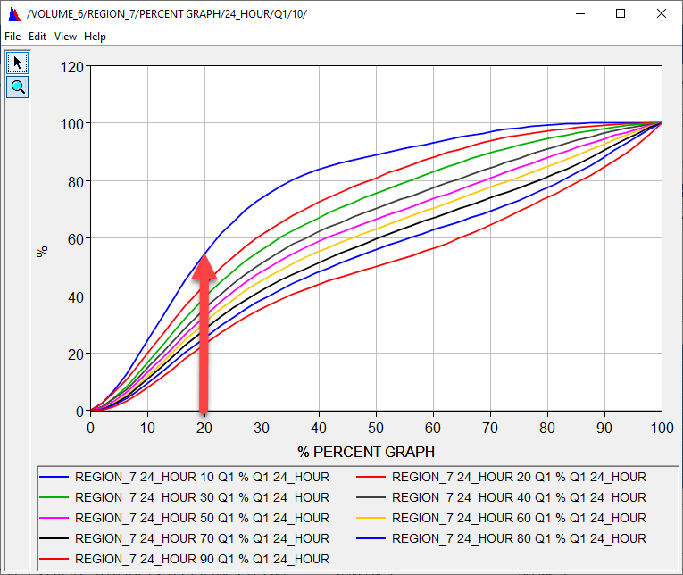
Part of the wealth of information available from Atlas 14 includes temporal patterns created from historical events. The temporal patterns are arranged based on the quartile of the storm the maximum precipitation fell. 1st quartile patterns are those patterns where maximum precipitation occurred in the first 6 hours for a 24-hour storm. Within each quartile, the historic time patterns are divided into percentage curves based on the cumulative hourly precipitation vs total storm precipitation. The following figure shows the 9 percent patterns within the 1st quartile storms for region 7 in California (the San Lorenzo River watershed falls within region 7). The figure shows that at 20 percent of a 24 hour storm (at 5 hours), 10 percent of the quartile 1 storms had already recorded more than 50 percent of the total storm precipitation.
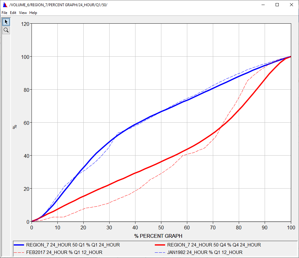
In this task you will import a 50 percent quartile 4 pattern from Atlas 14 and use this time pattern to compute an alternative set of flow-frequency values in the HEC-HMS model. The figure below shows the 24-hour 50-percent quartile 1 and 4 temporal patterns from Atlas 14 region 7 (solid blue and red lines). The blue dashed line is the percent time pattern from the January 1982 event that we used in this workshop. The red dashed line is the percent time pattern from the February 2017 event. The February 2017 event had its most intense precipitation near the end of the storm, which is consistent with a quartile 4 storm. Notice the precipitation intensity from the Feb 2017 event is higher than the 50 percent quartile 4 storm as indicated by the steeper slope in the cumulate percent pattern.
- Download the following HEC-DSS file and place it in your HEC-HMS project's Data folder - Atlas14TemporalPatterns.dss. This DSS file contains 24-hour Atlas 14 temporal patterns for region 7 in California.
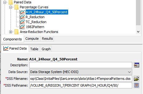
- Create a copy of the 1982Pattern percentage curve and name the copy A14_24hour_Q4_50Percent.
- Open the Component Editor for the new percentage pattern and change the Data Source to Data Storage System (HEC-DSS). Use the file chooser to locate the Atlas14TemporalPatterns DSS file that you copied to the project's Data folder. Then use the pathname chooser to select the Q4 50 percent pattern as shown in the figure below.
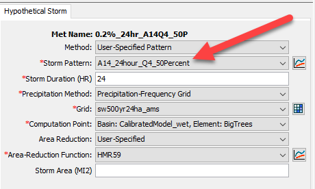
- Create a copy of the 0.2%_24hr_1982Pattern meteorologic model and name the copy 0.2%_24hr_A14Q4_50P. After you create the copy, change the storm temporal pattern so that the Atlas 14 time pattern is selected as shown below.
- Follow step 4 and create copies of the remaining hypothetical storms and update the copies to use the Atlas 14 time pattern.
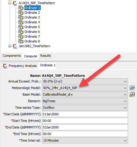
- Create a copy of the Jan1982_TimePattern Frequency Analysis compute. Name the new frequency analysis A14Q4_50P_TimePattern.
- Update each ordinate within the A14Q4_50P_TimePattern Frequency Analysis so that the correct meteorologic model is used. The figure below shows Ordinate 1 was updated to use the 50%_24hr_A14Q4_50P meteorologic model.
- Run the A14Q4_50P_TimePattern Frequency Analysis. Copy and paste the computed peak flow values into the highlighted cells in Column N on the Data tab in the FlowFrequencyPlot_HMR59 spreadsheet. The updated plot should look like the figure below.
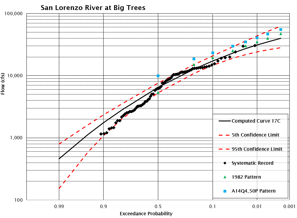
Notice how the flow-frequency values from the 50 percent quartile 4 temporal pattern are higher than results when using the 1982 temporal pattern. For most cases, storms with the heaviest precipitation located at the end of the event will generate higher flood flows than storms when the heaviest precipitation is located near the beginning of the event because initial losses (soil infiltration included) are generally higher at the beginning of a precipitation event.
The results from this analysis highlight a couple of key points.
- An HEC-HMS model can be used as a tool for developing flow-frequency relationships.
- The temporal pattern is a critical component when using a hydrologic model to simulate a flow-frequency relationship. Utilize historical storms and other information, like temporal patterns in Atlas 14, to build a sample of possible temporal patterns.
- The workshop did not attempt to incorporate uncertainty in initial conditions and other modeling parameters / assumptions. You could configure additional simulations where different area-reduction relationships were used and differ subbasin parameter and initial conditions are specified. HEC-HMS does have an uncertainty analysis compute options where some initial conditions and model parameters can be sampled in a Monte Carlo compute.
- The analysis assumed a one to one relationship between precipitation frequency and flow frequency. The 1-percent precipitation could fall on a wide range of initial conditions (soil moisture states).
Other considerations:
- Should the Calibrated model be adjusted, increase loss rates, to improve the fit between the HEC-HMS derived flow-frequency values and the Bulletin 17 flow-frequency curve?
- How do you choose one set of storm characteristics and basin model parameters for a representative model?
| Final Workshop Files | |
|---|---|
| HEC-HMS Project | |
| HEC-SSP Project | |
| Flow-Frequency Curve Spreadsheet | |