Task 2: Calibrate Snowmelt Parameters

Now that you've run the simulation and reviewed the results, try modifying the temperature index snowmelt parameters that control how snow accumulates and melts within the model. 

1. Open the Snowmelt plot for the Ouleout_S40 subbasin element, shown below.
   
   
2. Open the Snow Component Editor for the Ouleout_S40 subbasin element. The Component Editor will resemble the following figure.
   
   
   
   

   The PX Temperature is used to discriminate between precipitation falling as rain or snow. When the air temperature is less than the PX Temperature, any precipitation is assumed to be snow. When the air temperature is above the PX Temperature, any precipitation is assumed to be rain. Typical PX Temperature values range between 32 and 36 deg F.

   The difference between the Base Temperature and air temperature defines the temperature index used in calculating snowmelt. The wet/dry meltrate is multiplied by the difference between the air temperature and base temperature to estimate the snowmelt amount. If the air temperature is less than the base temperature, then the amount of melt is assumed to be zero. Typical Base Temperature values range between 32 and 36 deg F.

   The Wet Meltrate is used to define the rate at which the snowpack melts when air temperatures are greater than the base temperature and the precipitation rate exceeds a defined limit (i.e. Rain Rate Limit). Typical Wet Meltrate values range from 0.01 – 0.2 inches / deg F-day.

3. Modify the PX Temperature, Base Temperature, and Wet Meltrate values.
4. Compute the Forecast alternative and compare the updated SWE results to results from SNODAS for the Ouleout_S40 subbasin.
5. Adjust the parameters and rerun the simulation until an acceptable fit has been achieved between the computed and observed SWE data.
6. Repeat this process for the Treadwell_S10, Ouleout_S30, and Ouleout_S20 subbasins. A Temperature Index global parameter editor is available. As shown below, you can filter the table to only show subbasins upstream of the EastSidney_IN computation point. Also, you can choose the EastSidney_IN computation point in the bottom left part of the global editor and the program will only compute elements upstream of the selected location. 
    
   

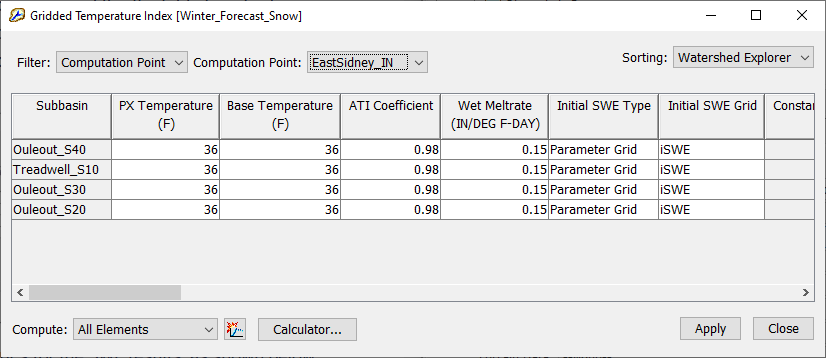
   The columns can be dragged to be in an order more advantageous to the user. In the above example image, the columns of concern for calibration purposed have been dragged next to the subbasin names. 

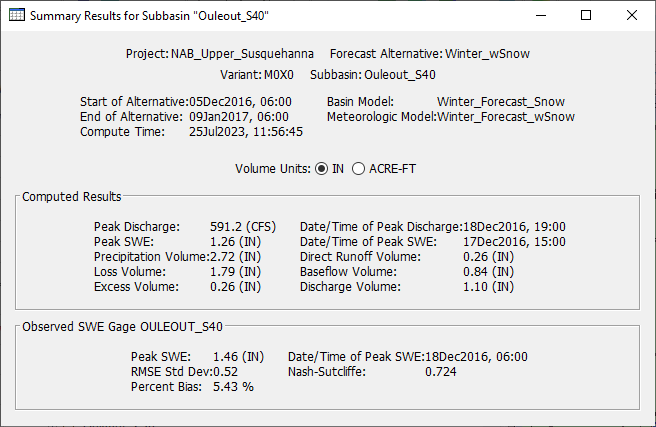
7. The subbasin summary table includes performance metrics for the SWE results, as shown below.