Task 3: Calibrate Other Precipitation-Runoff Parameters

As you should have noticed in the previous steps, the computed results do not exactly match the observed data during the lookback period. To improve the appropriateness of the forecast period, model parameters should be modified to provide a better match during the lookback period.

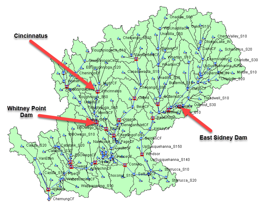
You will now calibrate precipitation-runoff model parameters to better match the observed data during the lookback period at three locations: Cincinnatus, WhitneyPoint_IN, and EastSidney_IN. The location of these elements are shown in the following figure. These three locations encompass the contributing drainage areas to each of the two NAB dams in the Upper Susquehanna River watershed.

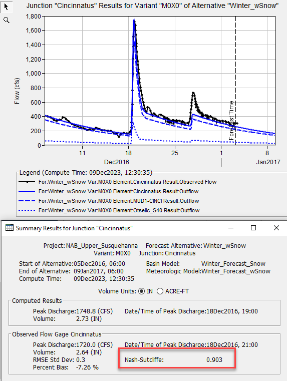
1. Compare the computed results at the Cincinnatus junction/gage location. Use the Graph and Summary Results table to view the computed and observed hydrographs as well as the associated statistical "goodness of fit" parameters.
2. In order to more accurately estimate inflow to Whitney Point Dam during a large event, it is important to first calibrate at Cincinnatus before proceeding downstream. While the initial estimates provide a decent place to start, the computed flow at this stream gage location does not adequately match the observed flow. Specifically, baseflow recedes too fast and storm runoff is under estimated when compared against the observed data. Therefore, the model parameters for the linked elements upstream of the gage need to be modified.
3. Keep the Graph for Cincinnatus open and viewable on your desktop window. Then, begin modifying the Recession Baseflow parameters for the subbasin elements upstream until an adequate baseflow recession is achieved. Open the Baseflow Zonal Editor by selecting Compute | Forecast Parameter Tables | Baseflow: Recession. Then, modify the Recession Constant adjustment factor for the Cincinnatus zone. Since this adjustment was defined as a specific value, the input parameter value replaces the old parameter value for the entire zone. Since baseflow recedes too quickly, you'll need to increase the Recession Constant. Type 0.925 within the Recession Constant Adjustment for the Cincinnatus Zone and hit Apply, as shown in the following figure.
   
4. In the lower left corner of the zonal modification editor, select the Cincinnatus computation point and click the Compute button. This is equivalent to using the Compute to Point (only compute elements which are upstream of the selected element).
5. Notice the changes to the runoff hydrograph at the Cincinnatus junction. The baseflow recession should now match the observed data much more closely than the initial computation.
6. Next, modify the initial deficit and constant loss rate parameters for the subbasin elements upstream until an adequate runoff volume and peak flow rate is achieved. Focus on the initial deficit first, you might not need to adjust the constant loss rate. 
7. Back to baseflow, you can improve the baseflow portion of the hydrograph on December 20 by increasing the ratio to peak parameter to 0.25 for all subbasins. 
8. Try to match the observed flow rates to achieve a Nash-Sutcliffe efficiency greater than 0.75.
   
9. Once you are satisfied with the calibrated results at the Cincinnatus junction, proceed to the WhitneyPoint_IN junction. The WhitneyPoint_IN Zone will need to be modified in a similar manner to achieve an adequate fit to the observed data for the lookback period. You will also need to adjust the initial baseflow for subbasins in the WhitneyPoint_IN zone to improve results at the beginning of the simulation.
10. Once you have adequately calibrated to the observed data at the WhitneyPoint_IN junction, move onto the EastSidney_IN junction.
11. The observed stage at Whitney Point Lake (and East Sidney Lake) should be used as a calibration target, not just the computed inflow. Computed inflow at each USACE-built dam is indirectly measured and based upon changes in pool stage and/or storage, outflow, and elevation-storage relationships. Therefore, effort should be given to matching observed pool elevation, which is directly measured.
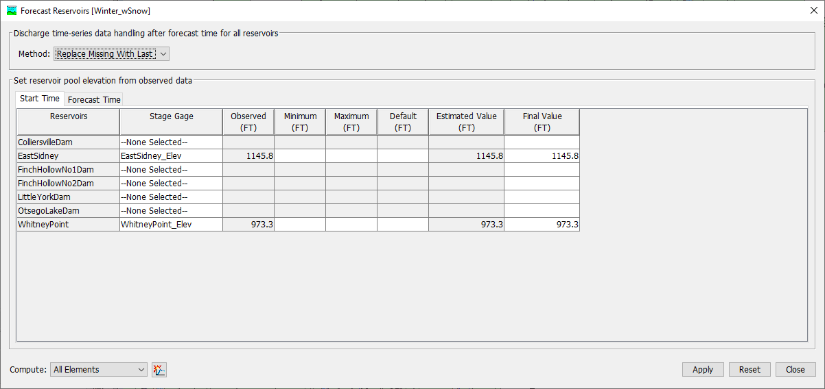
12. You will need to change the Initial Elevation for WhitneyPoint reservoir from 966.15 ft to 973.3 ft before comparing simulated and observed reservoir elevation. Change the initial elevation from 1139.3 ft to 1145.8 ft for the EastSidney reservoir.
    1. The Forecast Reservoirs editor can be used to automatically set the initial elevation at the beginning of the simulation to values in a stage time-series gage. You can also reset the reservoir elevation at the time of forecast. There are additional options for handling computed outflow during the forecast period.