Download PDF
Download page Applying Depth-Area Analysis to Precipitation-Frequency Grids.
Applying Depth-Area Analysis to Precipitation-Frequency Grids
Introduction
HEC-HMS version 4.6 has new features that support precipitation-frequency based rainfall-runoff modeling:
- A new "Precipitation-Frequency Grid" data type
- Capability to import ASCII-raster format grids to populate the Precipitation-Frequency Grid
- The Hypothetical Storm precipitation method of the meteorologic model can use a Precipitation-Frequency Grid as the source for precipitation depths
- The Hypothetical Storm precipitation method with a Precipitation-Frequency Grid can be used in the Depth-Area Analysis simulation type
This guide will provide information useful for creating an HEC-HMS model that allows you to perform hydrologic simulations with precipitation boundary conditions created by using precipitation-frequency grids. For most of the United States, the primary source of precipitation depth-duration-frequency data is NOAA Atlas 14, with the exception of the northwestern US. Depth-duration-frequency information for Washington, Oregon, Idaho, Montana, and Wyoming with similar coverage to Atlas 14 is a combination of data from Arkell and Richards (1986), NOAA Atlas 2, and TP-49. Other studies covering this region have been performed, such as Schaefer and Barker (2005) for Oregon, or Schaefer et al., (2006) for Washington (not an exhaustive list.) Atlas 14 contains frequency estimates for precipitation durations ranging from 5-minute to 60-day totals, and for frequencies from 1/2 AEP to 1/1,000 AEP. Additionally, Atlas 14 produces grid data that shows the depth at any point in the study area for a selected duration and frequency. NOAA Atlas 2 produces similar grids, except only for the 1/2 and 1/100 AEP frequencies and 6-hour and 24-hour durations.
Products such as Atlas 14 are point precipitation frequency products, meaning the grid is a representation of the depth-duration-frequency relationship for a single point in space. The pattern in a grid of point precipitation frequency values is not realistic for an actual storm event because it assumes the same frequency event (e.g. a 1% AEP 24-hour storm) is occurring at all locations simultaneously. Typically, depth-area reduction is used to adjust point values to area-averaged values. A depth-area reduction curve expresses the amount by which the area-averaged precipitation decreases from the point (or 10 mi2) maximum value for storm events. They may be derived from a single storm, or by generalizing several storm events. The area component of a depth-area reduction refers to the overall area, or footprint, of the storm. For hydrologic simulations, a frequently-made simplifying assumption is to set the storm area equal to the drainage area of the watershed above the location being analyzed. Analyses that consider multiple locations then have a varying drainage area and therefore storm area, which changes the area reduction factor for computing area-averaged precipitation. The Depth-Area Analysis in HEC-HMS automatically handles this operation.
The HEC-HMS model you are using must be georeferenced, either by creating the basin model using the HEC-HMS delineation tools, by importing georeferenced elements, or by georeferencing an existing model.
Consider reviewing the Applying the Depth Area Analysis Simulation Type tutorial for additional details on using the Depth-Area analysis.
Preparing Input Data
Three critical inputs to this process are the Precipitation-Frequency Grid, the Storm Pattern, and the Area Reduction Function.
Precipitation-Frequency Grid
The Precipitation-Frequency Grid data type in HEC-HMS was designed with seamless integration of NOAA Atlas 14 grids in mind. Other grids can be used as well, such as NOAA Atlas 2, or user-created grids. Atlas 14 grids can be acquired using the NOAA HDSC Precipitation Frequency Data Server, and are delivered in ASCII raster format. Atlas 14 and Atlas 2 grids are floating-point data stored as integers by means of a "scale factor." Always check the metadata for the data scale factor. Generally, Atlas 14 depths are stored by taking the floating-point value and multiplying by 1,000 (meaning the units of the grid are 1/1,000 inch.) Atlas 2 depths are generally stored by taking the floating-point value and multiplying by 100,000 (meaning the units of the grid are 1/100,000 inch.)
ASCII rasters are a text-based raster format characterized by a 6-line header describing the spatial extents, resolution, and no-data value of the dataset, and delimited text values representing the raster values in the body (see Figure 1.) Typically these files are accompanied by a ".prj" file of the same name that defines the spatial reference used in the header.
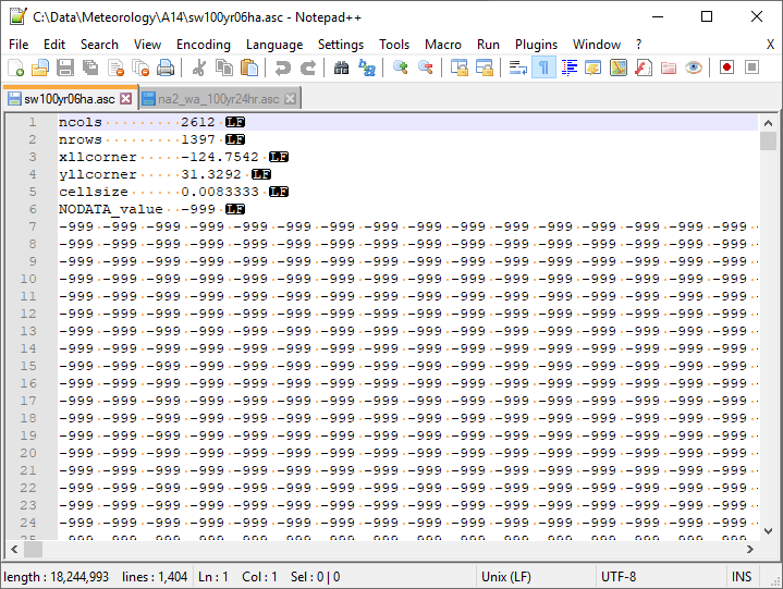
Figure 1. ASCII-format raster file example.
After acquiring the desired depth-duration-frequency grid, create a new Grid Data shared data component by choosing Components > Create Component > Grid Data... (Figure 2)
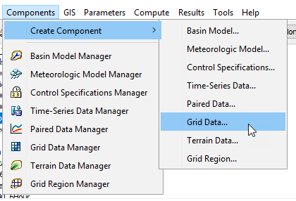
Figure 2. Creating a grid data component.
This will launch a dialog box that allows you to name and set the data type for the new Grid Data. A convention is to use the standard filename from Atlas 14 or Atlas 2 (if those are the data source) for the grid name, as this encodes the study area, AEP, duration, and type of analysis that create the dataset. Choose the "Precipitation-Frequency Grids" data type (Figure 3).
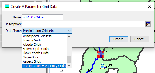
Figure 3. Creating a Precipitation-Frequency Grid.
This will create a new Precipitation-Frequency Grid in the Watershed Explorer. Select it in the tree to launch the editor (Figure 4.) By default, the data source will be set to Single Record HEC-DSS. Change this to ASCII.
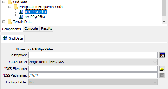
Figure 4. Default Grid Data component editor.
The settings for an ASCII grid include the filename, units for the grid, and scale factor (Figure 5.)
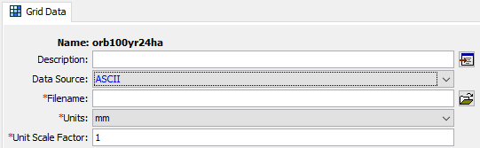
Figure 5. ASCII grid component editor.
Choose the path to the ASCII raster grid (.asc file) for Filename. Check the metadata for units and scale factor. Atlas 14 is typically "in" and "1000", and Atlas 2 is typically "in" and "100000". User-created datasets may be different. A fully-parameterized grid will look like Figure 6.
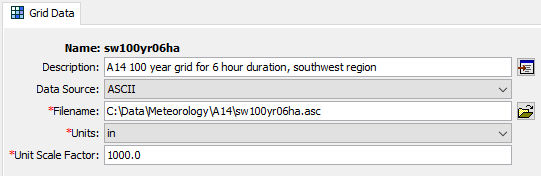
Figure 6. Parameterized Precipitation-Frequency Grid.
Storm Pattern
The Storm Pattern describes the distribution of rainfall depth in time. In HEC-HMS and they are entered as Paired Data components with the "Percentage Curves" type (Figure 7.) Usually these patterns are supplied as dimensionless storm patterns (dimensionless mass curves.) The time component is the percent of the total duration of the storm event. The depth component is the percent of the total depth of the storm. One common source of time patterns is the Atlas 14 Temporal Distributions, which has dimensionless patterns derived from 6-, 12-, 24-, and 96-hour duration storm events.
Storm Patterns are created by selecting Components > Create Component > Paired Data... and selecting the "Percentage Curves" data type.
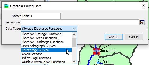
Figure 7. Creating a Percentage Curve Paired Data component.
After creating the Percentage Curve, select it in the Watershed Explorer to open the editor. Values can be set using Manual Entry (the default) or HEC-DSS. Manual Entry allows the user to enter the storm percent of duration (first column) and storm percent of total depth (second column) and can be copied and pasted from spreadsheet software. The values in both columns must be strictly increasing and the last value must be 100 (Figure 8.)
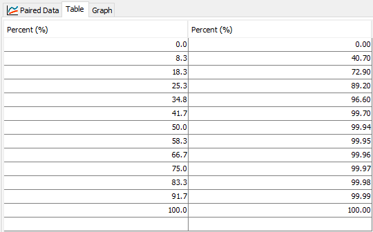
Figure 8. Entering a Percentage Curve for a Storm Pattern.
The pattern can be viewed as a mass curve graph by selecting the Graph tab (Figure 9.) The curve shown below is a front-loaded storm, where most of the precipitation occurs in the first 25% of the storm.
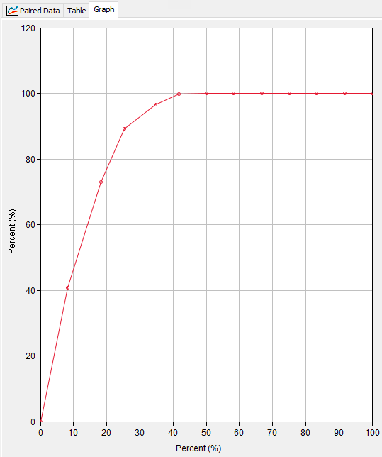
Figure 9. Graph of percentage curve.
Area-Reduction Function
Area-reduction functions describe the relationship between the point maximum precipitation observed in a storm pattern, and the average depth of precipitation averaged over a larger area. It is a highly-idealized means of describing the spatial pattern of precipitation in space. It accounts for the decrease in average storm intensity over larger areas.
In HEC-HMS area reduction functions are a type of Paired Data curve and can be created using the Components > Create Component > Paired Data... menu option and selecting the Area-Reduction Functions data type. There are two ways to import Area-Reduction information: manual entry (the default) and HEC-DSS. Manual entry allows the user to enter values in a two-column table corresponding to the storm area (in km2 or mi2) and the reduction factor (a value less than 1; see Figure 10.) Area reduction factors decrease as storm area increases (Figure 11, a graph view of the user-entered Area-Reduction Function.)
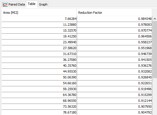
Figure 10. Tabular entry of an Area-Reduction Function.
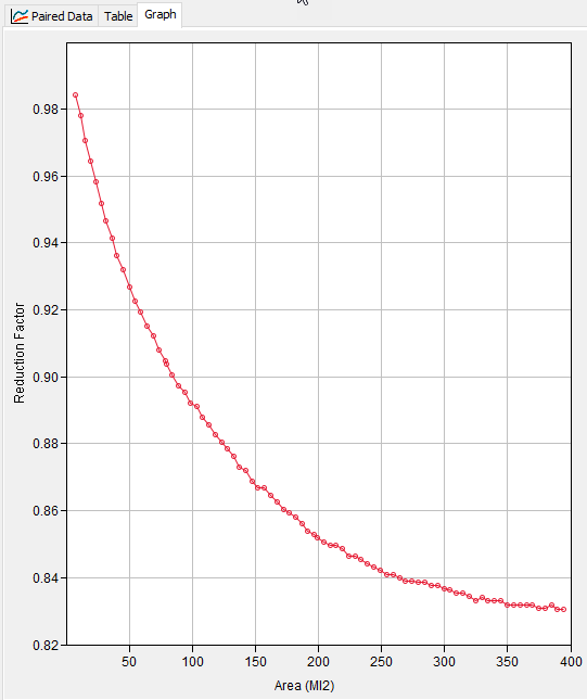
Figure 11. Graph view of a user-entered Area-Reduction Function.
Setting Up the Meteorologic Model
Create a new Meteorologic Model by choosing Components > Create Component > Meteorologic Model... and open the editor by selecting the Meteorologic Model in the Watershed Explorer. Choose the Hypothetical Storm method for precipitation in a Meteorologic Model. Set the Meteorologic Model to be able to use the basin model of interest by selecting the Basins tab and setting "Include Subbasins" to "Yes" for the basin model. Open the Hypothetical Storm editor by selecting it in the Watershed Explorer beneath the Meteorologic Model. Set the Method to User-Specified Pattern, and the Precipitation Method to Precipitation-Frequency Grid (Figure 12.)
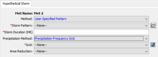
Figure 12. Hypothetical Storm options that enable using the Precipitation-Frequency Grid selected.
Next, set the Storm Pattern in the drop-down to the pattern entered previously. If the pattern entered previously is not available, check to make sure it was entered as a Percentage Curve.
Then, set the storm duration equal to the duration specified in the Precipitation-Frequency Grid.
Next, set the Grid to the Precipitation-Frequency Grid created previously.
Finally, set the Area Reduction method. The TP-40 area reduction curve is available, but if you choose to use it, should only be used with 24-hour duration storms. If you choose the User-Specified option, you will need to supply an area-reduction function (created as a Paired Data component with the Area-Reduction Function type.) Once an area reduction method is set, the option to set a Computation Point becomes available. This point will be used to compute the storm area but will be overridden by analysis points in the Depth-Area Analysis. If this Hypothetical Storm is used in a regular Simulation Run, it will use the storm area corresponding to the drainage area above this computation point. A fully-parameterized Precipitation-Frequency Grid Hypothetical Storm is shown in Figure 13.
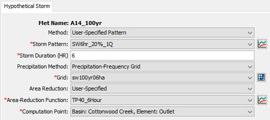
Figure 13. Fully-parameterized Hypothetical Storm with Precipitation-Frequency Grid.
Setting Up the Depth-Area Analysis
Create a new Depth-Area Analysis by selecting Compute > Create Compute > Depth-Area Analysis... A wizard will appear. Enter a name on the first prompt and select "Next >". Then, select the appropriate Basin Model and select "Next >". Then, select the Meteorologic Model that employs the Hypothetical Storm, and select "Finish." Switch to the "Compute" tab in the Watershed Explorer and select the Depth-Area Analysis that was just created, to open the editor (Figure 14).
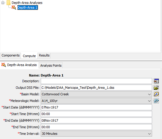
Figure 14. Editor for the Depth-Area Analysis.
Enter a start and end date and time that gives enough time for the entire hydrologic response for the watershed to pass; at minimum, set the total simulation duration as long as the storm duration. Choose an appropriate time interval for the simulation. Then, switch to the Analysis Points tab (Figure 15.) On this tab, any element in the Basin Model can be added for analysis to the right column of the table. The Depth-Area Analysis, when it runs, will iterate over this list of elements. For each element, the Depth-Area Analysis will compute the drainage area above the Analysis Point, compute the area average of the Precipitation-Frequency Grid in the Meteorologic Model above the Analysis Point, compute the depth-area reduction factor from the area reduction curve in the Meteorologic Model, reduce the area-averaged precipitation-frequency depth using the computed factor, distribute the reduced depth in time using the Storm Pattern, and execute a hydrologic simulation. If three analysis points are entered, three hydrologic simulations will execute.
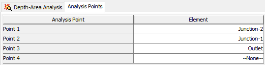
Figure 15. Analysis points in the Depth-Area Analysis.
If displaying note messages in the console is enabled, each iteration will report the storm area, area-averaged precipitation depth, and hypothetical storm area in the console (Figure 16).
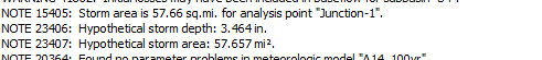
Figure 16. Depth-Area Analysis reporting in the console.
Viewing Results
Switch to the Results tab and select the Depth-Area Analysis in the Watershed Explorer. Beneath the Depth-Area Analysis, a table displaying a Peak Flow Summary will be shown, as well as a folder icon for each of the selected analysis points (Figure 17.)
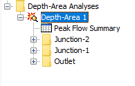
Figure 17. Depth-Area Analysis results in the Watershed Explorer.
Selecting the Peak Flow Summary table will display a table with each analysis point, the drainage area, and the magnitude and time of the peak discharge for the simulations (Figure 18.)
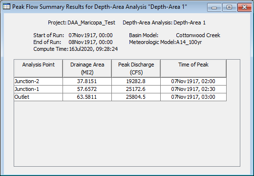
Figure 18. Peak Flow Summary table for Depth-Area Analysis.
Expanding the menu for one of the analysis points allows you to view the time-series results at each element in the simulation targeted for each analysis point.