Sampling Depth-Area-Reduction Curves for a Hypothetical Storm

For more background on depth-area-reduction curves and their use with frequency simulation options refer to Applying the Frequency Storm Met Model in HEC-HMS and Applying the Hypothetical Storm Met Model in HEC-HMS. You can also practice stochastic sampling of NOAA Atlas 14 temporal storm patterns.

Software Version

HEC-HMS version 4.12 was used to create this tutorial. 

This tutorial should take approximately 30 minutes to complete.

Download the initial project files here:

Area_Reduction_Sampling_HMS_Initial.zip

Introduction

When applying a point precipitation to a watershed, such as the case with Frequency Storm and Hypothetical Storm simulation in HEC-HMS, depth-area-reduction factors are required to reduce the point precipitation depth to an average depth that occurs over the watershed. The general relationship is that average rainfall depth decreases with an increase in storm area. However, the exact magnitude of decrease varies between storms and locations. Therefore, there is an uncertainty associated with the selection of depth-area-reduction relationship. 

In this tutorial, you will use Uncertainty Analysis in HEC-HMS to randomly sample from a selection of depth-area-reduction curves derived from from historic storms in NOAA’s Hydrometeorological Report No. 51 (HMR 51). You will evaluate how the uncertainty in depth-area-reduction curve influences the modeled flow results for a 1/100 annual exceedance probability and the 4-day (96-hr) duration hypothetical storm.

Study Area

You will continue using the HEC-HMS model developed in the Hypothetical Storm workshop for the Village Creek watershed. This watershed is located near Beaumont, Texas in the southeastern portion of the state and is approximately 1,130 square miles, as shown in the location map below. The hypothetical storm in this simulation was derived by combining the precipitation-frequency grid for 1/100 annual exceedance probability and 4-day duration with the temporal pattern of a historical storm that occurred in October 2006.

Data

Depth-area-reduction relationships used in this workshop were developed from depth-area-duration information in NOAA’s Hydrometeorological Report No. 51 (HMR 51, https://www.weather.gov/owp/hdsc_pmp). The historic storms contained in HMR 51 were influential in setting the level of Probable Maximum Precipitation (PMP) for the Eastern U.S. Below is the figure from HMR 51 showing the locations of the more influential storms used to develop PMP index maps. 

The figure below shows an example of the depth-area-duration table from the Appendix of HMR 51 for one of these storms. See the workshop on Creating Depth-Area Reduction Curves from Gridded Precipitation Data to learn how to compute Depth-Area Duration (DAD) tables from the observed gridded precipitation data.

For this workshop, depth-area-reduction relationships were already added to the project's Paired Data for all the individual storms with 96-hour duration (to match the duration of the hypothetical storm in the model), as shown in the figure below. You can consult the workshop on Applying the Frequency Storm Met Model in HEC-HMS for step-by-step instructions on how to develop storm-specific depth-area-reduction curves from the DAD tables. 

Most of the storms used to develop area-reduction curves in this workshop are not in the area of the watershed. However, for workshop purposes, a variety of storms was used to emphasize the impact of variability in the area-reduction functions. In reality, you may want to use multiple historic storms near your location to develop area-reduction relationship.

Examine area reduction curves

Open Village_Creek.dss file in Project folder. Select AREA-REDUCTION-FACTOR under Part C drop down box, select all the area-reduction curves that were added in this example (exclude the first one titled Local_96hr_100yr) and click Select button. 

Click on the graph icon in the toolbar to display the curves. You can right-click and modify the the display axes to match the figure below.

Question: What range of reduction factors do you expect from these curves for the meteorological model in this project.

Create a Parameter Value Sample

Parameter Value Sample tables provide a list of parameter values that can be sampled randomly or in a specified order as part of the Uncertainty Analysis. Starting with version 4.12, Parameter Value Sample tables can contain names referencing other paired data functions. HEC-HMS currently supports sampling of storm grids, storm patterns (see Sampling NOAA Atlas 14 Temporal Patterns) and area-reduction curves. The process of creating a Parameter Value Sample for storm patterns and grids has been expedited with the Parameter Value Sample Creator wizard. For now, you will need to manually enter depth-area-reduction functions into the Parameter Value Sample table. An Excel file with the curve names has been added to project files to speed up this process.

Open the Paired Data Manager from Components | Paired Data Manager. Scroll down to select Parameter Value Samples data type, as in the figure below.

Click on the New button and name the new table All curves. 

Open the new table by expanding the Paired Data node and clicking on the table name in the project tree. Select Data Source: Manual Entry, Method: Hypothetical Storm and Parameter: Area-Reduction Function. Your selections should match the figure below.

Now click on the Table tab to add the names of the 17 area-reduction functions listed under the Paired Data | Area Reduction Functions node. To save time, you can copy all the function names from the included Excel spreadsheet and paste them by right-clicking on the first cell of the table and selecting Paste. 

Run Uncertainty Analysis with all area-reduction functions

Refer to Uncertainty Analysis Simulations in HEC-HMS workshops if needed. Browse to Compute | Uncertainty Analysis Manager and click New to create a new Uncertainty Analysis and name it Uncertain area reduction. Add the basin model and met model.

Go to the Compute tab and select the new Uncertainty Analysis you created. Set Start Time, End Time and Time Interval to match the settings in Control Specifications. Include all analysis points and set the number of samples to 50 to save time.  HMS will automatically choose a random seed for you.

Right-click on the Uncertain area reduction Uncertainty Analysis to add a parameter. Select the newly added Parameter 1 node. Choose Element: –Precipitation Parameters--.  Select Parameter: Hypothetical Storm - Area-Reduction Function and Method: Specified Values - Random (Independently Random) then save your project. and choose the All curves Parameter Value table from the drop down menu. Your dialog should look like the figure below.

In the Uncertainty Analysis editor, choose the gear icon next to Analysis Points and select the NechesRv_Nr_Beaumont Outflow timeseries and press Save then Close.

Run the Uncertain area reduction Uncertainty Analysis. It will take approximately one minute. Examine the Uncertainty Analysis results for the NechesRv_Nr_Beaumont outlet. Your results may be slightly different from the ones in the figure below due to having a different random seed in the Uncertainty Analysis.

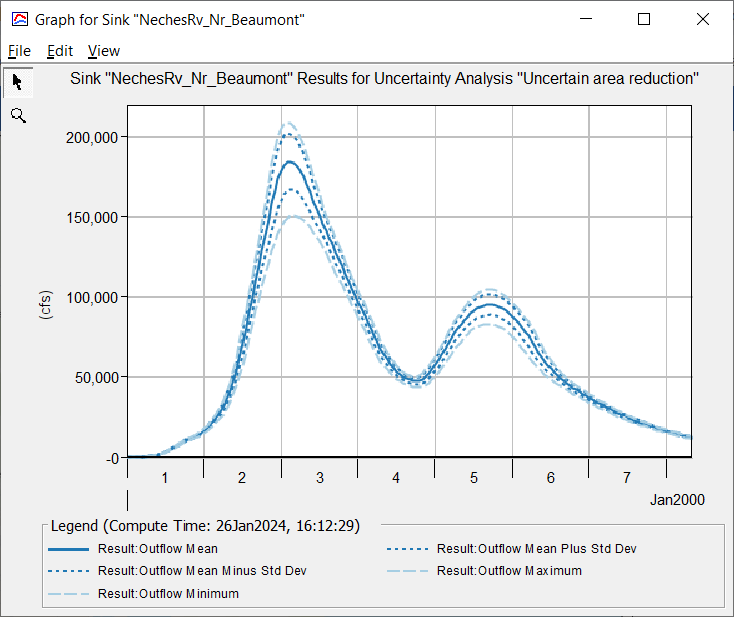
Question: use the Maximum Outflow Table in the Uncertainty results for this location to calculate maximum, minimum and mean peak flows.

Question: What physical factors could cause variability in the area reduction relationships for the 96-hr storm? How would you go about creating a more appropriate depth-area-reduction function for the watershed?

Project Files

Download the final project files here:

Area_Reduction_Sampling_HMS_Final.zip

References:

Olivera, Francisco & Asce, M & Choi, Janghwoan & Kim, Dongkyun & Li, Ming-Han. (2008). Estimation of Average Rainfall Areal Reduction Factors in Texas Using NEXRAD Data. Journal of Hydrologic Engineering. 13. 10.1061/(ASCE)1084-0699(2008)13:6(438).