Download PDF
Download page Storm Parameter Variability.
Storm Parameter Variability
Last Modified: 2025-07-21 16:13:42.293
Overview
The Hypothetical Storm method is a widely used meteorological approach for generating design storms. Key storm parameters considered in this method include:
- Depth
- Temporal Pattern
- Area Reduction
- Spatial Distribution
This guide focuses on demonstrating the variability of the first three parameters. Storm depths are determined using NOAA Atlas 14 precipitation-frequency grids, considering the median as well as the 5% and 95% confidence limits. Variability in temporal patterns and area reduction factors is analyzed using gridded rainfall data from Multi-Radar Multi-Sensor (MRMS) Quantitative Precipitation Estimates for recent events, and Analysis of Record Calibration (AORC) for older events. Gridded storm data are then converted to basin-average time series for further analysis. Additionally, historical storm patterns are compared to the hypothetical storm patterns derived from NOAA Atlas 14 as well as a sensitivity analysis was also conducted on storm duration to identify the duration that generates the maximum peak flow.
Software Version
HEC-HMS version 4.13 was used to create this tutorial. You will need to use HEC-HMS version 4.13, or newer, to open the project files.
Project Files
Download the initial files here:

Excel File:
Temporal Pattern DSS File: StormPattern.dss
Areal Reduction DSS File: AreaReduction.dss
HEC-HMS Model
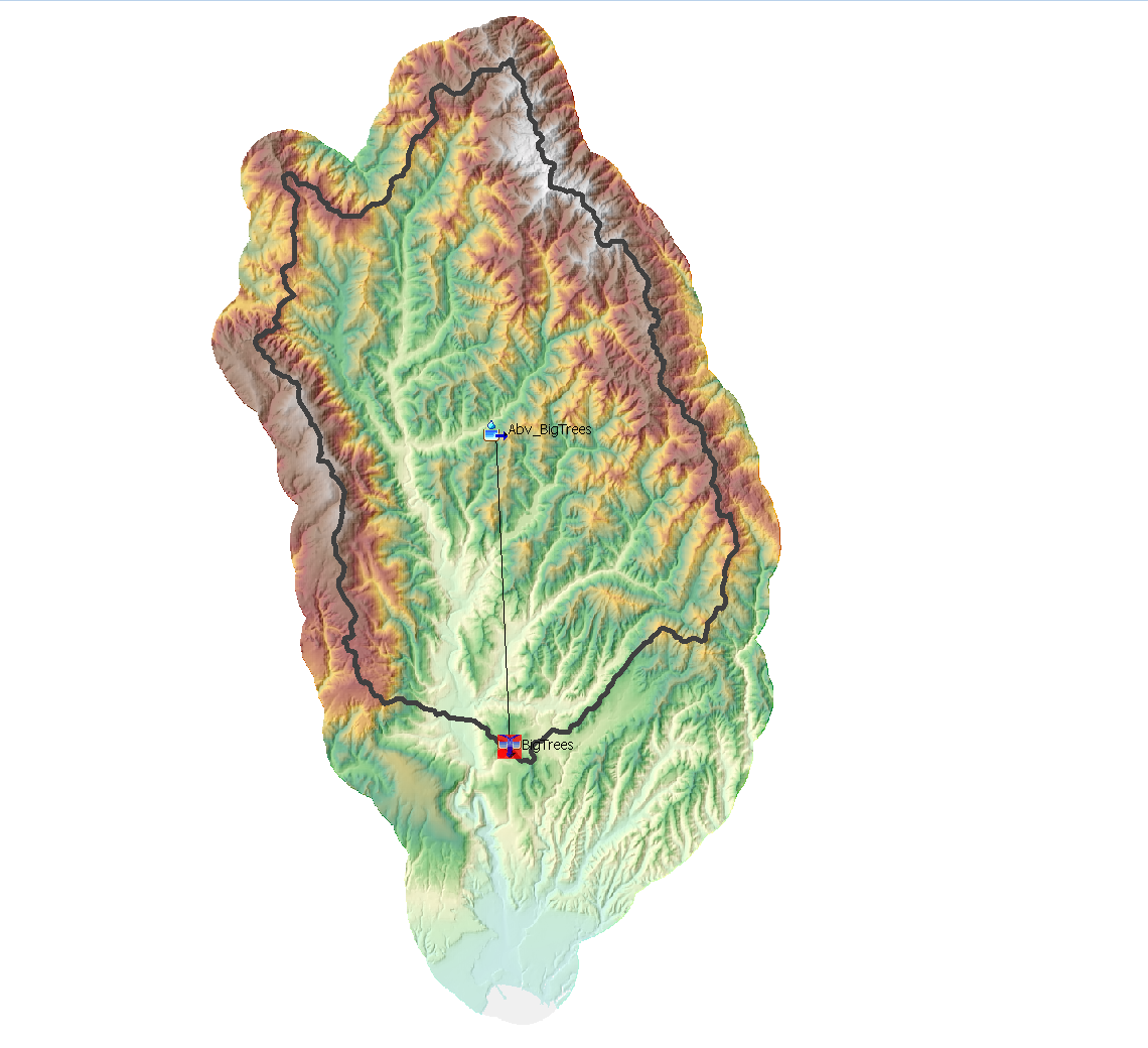
This model was originally obtained from this tutorial: Modeling Flow-Frequency Relationships using HEC-HMS. The watershed area was delineated starting from the San Lorenzo River gage location using the delineation features in HEC-HMS. The watershed is represented as a single basin.
Basin processes used in the model are described in the table below.
Process | Methods |
|---|---|
| Loss | Deficit and Constant |
| Transform | Variable Clark Unit Hydrograph |
| Baseflow | Linear Reservoir Baseflow |
| Discretization | Structured |
| Meteorology | Gridded Precipitation |
Additional calibrations and refinements were included for this guide and included in the initial files.
Precipitation-Frequency Depths
For California (Volume 6) at the San Lorenzo watershed, the NOAA Atlas 14 documentation does not provide the exact statistical parameters used to fit the frequency curves, nor does it specify the equivalent record length (ERL) needed to quantify uncertainty. However, the documentation does indicate that the Generalized Extreme Value distribution provides an acceptable fit to the annual maximum series (AMS) data. For this analysis, the GEV distribution was assumed, and its moments were estimated through a root mean square error (RMSE) minimization process. Estimating the frequency curve process is described in more detail here: Hydrologic Sampler Setup.
Using the 500 realizations of the 48-hour precipitation frequency curves, the quantiles were extracted for the 50%, 10%, 4%, 2%, 1%, 0.5%, 0.2%, and 0.1% AEP where each quantile would have 500 rainfall depths. The spreadsheet provided contains rainfall depths for the specified quantiles. The Realization tab holds 500 48-hr precipitation-frequency curve created from the bootstrap Monte Carlo process. The Calc tab estimates the desired quantiles by linearly interpolating between the z-scores and rainfall depths. A scale and shift adjustment was further performed on the rainfall depths to better match the confidence range. A histogram was plotted of the original dataset against the shifted dataset to ensure the distribution remained consistent.
- In the Depths to Copy tab of the spreadsheet, copy the 10% column and add to HEC-HMS as a Parameter Value Sample.
- Navigate to the Components Menu and select Pair Data Manager. Select Parameter Value Samples as the Data Type.

- Click new and name the file 10percentAEP.
- Repeat this for the 2%, 1%, and 0.1% AEP.
- Expand Paired Data | Parameter Value Samples in the Watershed Explorer, and click on the 10percentAEP. Choose the following selections:

- In the Table tab, paste all of the depths in the 10% column in the Depths to Copy tab of the Excel spreadsheet. Repeat for the 2%, 1%, and 0.1% quantiles.
- Navigate to the Components Menu and select Pair Data Manager. Select Parameter Value Samples as the Data Type.
Temporal Patterns
The timing of peak rainfall within these patterns is often critical; placing the heaviest rainfall near the beginning, middle, or end of a storm can significantly alter peak flow predictions. For this analysis, the historic storm patterns that calibrated at least satisfactory are used and treated as a variable parameter. Temporal patterns were created for each storm for the 48-hr durations. HEC-HMS requires the temporal patterns to be created as Percent Patterns. Percent Patterns are Paired Data Types that take in a percent vs percent relationship. The maximum 48 hour period was used to create the temporal storm pattens. Creating a temporal pattern from an observe storm is described in this tutorial. The temporal patterns are provided as a HEC-DSS file.
- Download the StormPattern.dss file and save to the project data folder.
- Navigate to the Components Menu | Paired Data Manager and select Percentage Curves as the Data Type.
- Create a New Percentage Curve for the 1982 storm pattern.
- Navigate to the Paired Data | Percentage Curves in the Watershed Explorer. Select 1982-48hr Percentage Curve and select Data Storage System (HEC-DSS) as Data Source in the Component Editor. Select the StormPattern.dss file and choose the 1982-48hr in the DSS Pathname.

- Right click on 1982-48hr Paired Data and select Create Copy. Name the Paired Data 1998-48hr. In the Paired Data Component Editor, change the DSS Pathname to 1998-48hr. Repeat this process for 2016, 2017, 2019, 2023-1st, 2023-2nd, and 2023-3rd storm patterns.

- Navigate to Tools | Data | Atlas 14 | Parameter Value Sampler Creator to open the Parameter Value Sample Creator window. In the combo box select Storm Pattern. Select all of the storm patterns and click Next. Name the Parameter Value Sample AllTemporalStorms and click Next. Select Project DSS file and select Next to create the Parameter Value Sample.
- Navigate to the Parameter Value Samples in the Watershed Explorer and select AllTemporalPatterns. In the Component Editor Table tab, the following Values should appear.

Depth Area Reduction
In practice, generalized DARFs over regions have been created for modeling purposes, such as TP-40-49 and depth area functions in HMR documents. These curves are created from historic storms generalized for a given region. For this analysis, rather than use a generalized DARF, a unique DARF for each historic storm is created and treated as a variable parameter in the rainfall-runoff model. Storm-specific depth–area reduction curves were developed for each event that yielded "Satisfactory" calibration results, as these storms exhibited temporal patterns and depths that could closely reproduce observed hydrograph. The reduction curves were created using MetVue 3.2 and described in this tutorial. Setting up depth area reduction functions is described in this tutorial.
- Download the ArealReduction.dss file and save to your project data folder
- Navigate to the Components Menu | Paired Data Manager and select Area-Reduction Functions as the Data Type.
- Create a New Area-Reduction Functions and name the Paired Data 1982-48hr.

- Navigate to the Paired Data | Area-Reduction Functions in the Watershed Explorer. Select 1982-48hr Area-Reduction Function and select Data Storage System (HEC-DSS) as Data Source in the Component Editor. Select the AreaReduction.dss file and choose the 1982-48hr as the DSS Pathname.
- Right click on 1982-48hr Paired Data and select Create Copy. Name the Paired Data 1998-48hr. In the Paired Data Component Editor, change the DSS Pathname to 1998-48hr. Repeat this process for 2016, 2017, 2019, 2023-1st, 2023-2nd, and 2023-3rd storm patterns.
- Navigate back to the Components | Paired Data and Select Parameter Value Samples as the Data Type. Create a new Parameter Value Sample and name it AllAreaReductionFunctions. In the Watershed Explorer, select AllAreaReductionFunctions under Parameter Values Samples. Select the following methods in the Component Editor.

- Navigate to the Table tab and enter the names of the Percentage Curves Paired Data under Value.
TP-40-49 and HMR-59 depth area reduction curves are compared to storm areal reduction curves. Across most areas, TP-40-49 has a lower reduction than the historical storms while HMR-59 falls within the middle of the historical storms for larger areas. Given TP-40-49 was created over 50 years ago and uses storms across the U.S., regional depth area reduction curves such as HMR-59 matches local historic storms better.

Hypothetical Storm Meteorological Model
Hypothetical Storm Meteorological Model allows you to create design storms based off a single duration where the user needs to define the storm depth, storm pattern, depth areal reduction, and storm distribution. A tutorial on setting up a basic Hypothetical Storm is described in this tutorial. The Uncertainty Analysis compute will work with the Hypothetical Storm Meteorological Model.
- Navigate to Components | Meteorologic Model Manger to create a new Met Model. Name the first model 10percentAEP. Create 3 more models with the names 2percentAEP, 1percentAEP, and 0.1percentAEP.
- Head over to Meteorologic Models in the Watershed Explorer and expand 10percentAEP model. Change the Precipitation Method to Hypothetical Storm.

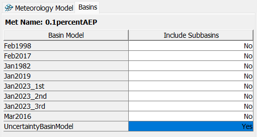
- In the Basins tab, make sure the UncertaintyBasinModel has the Include Subbasins selected to Yes.
- In the Hypothetical Storm Component Editor, keep the Method as User-Specified Pattern, set the Storm Duration to 48, the Spatial Distribution to Uniform for All Subbasins, the Precipitation Method as Point Depth, the Area Reduction as User Specified, and the Storm Area to 106.63. Choose any Storm Pattern, Point Depth, and Area-Reduction Function since these will be sampled from the Parameter Value Sample.

- Repeat this for the other three Meteorologic Models. Ensure you have the UncertaintyBasinModel Include Subbasins selected to Yes.
Uncertainty Analysis Compute
The Uncertainty Analysis Compute uses a Monte Carlo sampling technique to sample from the rainfall depths, temporal patterns, and areal reduction functions.
- Navigate to the Compute | Uncertainty Analysis Manager and create a New Uncertainty Analysis with the name 10percentAEP
- Select the UncertaintyBasin as the Basin Model and 10percentAEP as the Meteorologic Model.
- Select 10percentAEP Uncertainty Analysis Component Editor, set a Start Date of 01Jan2025, a Start Time of 00:00, an End Date of 05Jan2025, and an End Time of 00:00. Leave the Time Interval as 1 Hour and set the Total Samples to 500. Leave the Seed Value.

- Select the cog wheel next to Analysis Points. In the Results window, select the checkmark box Abv_BigTrees - Precipitation Time-Series and BigTrees - Outflow Time-Series. Select Save and Close.

- Right click on 10percentAEP and choose Add Parameter. Repeat this two more times to create 3 Parameters.
- Select Parameter 1. Next to Element, select --Precipitation Parameters– and next to Parameter, select Hypothetical Storm - Point Depth. Next to Method, select Specified Values - Sequential Loop and next to Parameter Value choose 10percentAEP.

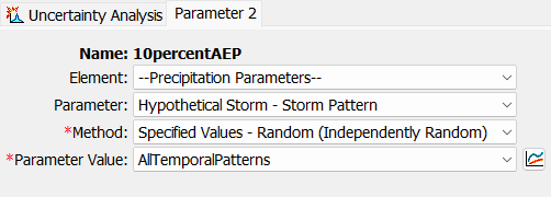
- Move onto Parameter 2. Next to Element, select --Precipitation Parameters– and next to Parameter, select Hypothetical Storm - Storm Pattern. Next to Method select Specified Values - Random (Independently Random) and next to Parameter Value select AllTemporalPatterns.
- Move onto Parameter 3. Next to Element, select --Precipitation Parameters– and next to Parameter, select Hypothetical Storm - Area-Reduction Functions. Next to Method select Specified Values - Random (Independently Random) and next to Parameter Values select AllAreaReductionFunctions.
- Right click on 10percentAEP and select Create Copy. Name the Uncertainty Analysis 2percentAEP. Repeat the copy for the 1percentAEP and 0.1percentAEP.
- For each copy of the Uncertainty Analysis, change Parameter 1 to the correct Parameter Value (i.e. 2percentAEP Uncertainty Analysis has the 2percentAEP Parameter Value)
- Head to Compute menu and select Multiple Compute. Switch the Compute Type to Uncertainty Analysis and Select All simulations. Click Compute to compute the Uncertainty Analysis. The compute time should take less than a 4 minutes to finish depending on the number or cores within your computer.
Results
The Uncertainty Analysis will save only the results that are specified in the Analysis Points. The selected parameters are saved as tables and can be viewed in the Results tab.
- Navigate to the Results Tab and expand the Uncertainty Analysis folder. Expand the 10percentAEP and select Parameter 1. This shows the selected precipitation depths. The Sample Number corresponds to the simulation order out of 500 events. Look through Parameter 2 and Parameter 3 to see the selected temporal patterns and areal reduction functions.
- Expand BigTrees node and select Maximum Outflow. This corresponds to the peak flow value for each depth, temporal pattern, and area reduction combination.
- Open the Histogram Results.xlsx file and copy all 500 Maximum Outflow Statistic Value to the Paste tab. Find the corresponding annual exceedance probability and paste the values. Navigate to the Box and Whisker - Histogram tab to view the results. The Box and Whisker shows the spread of the peak outflows along with the mean and median value for each quantile. The histogram provides a cross sectional view of the data for each quantile.


Continue to Frequency Depth Duration Comparison