Download PDF
Download page v.4.7.0 Release Notes.
v.4.7.0 Release Notes
Beta release:
Final release:
New Features
2D Diffusion Wave transform
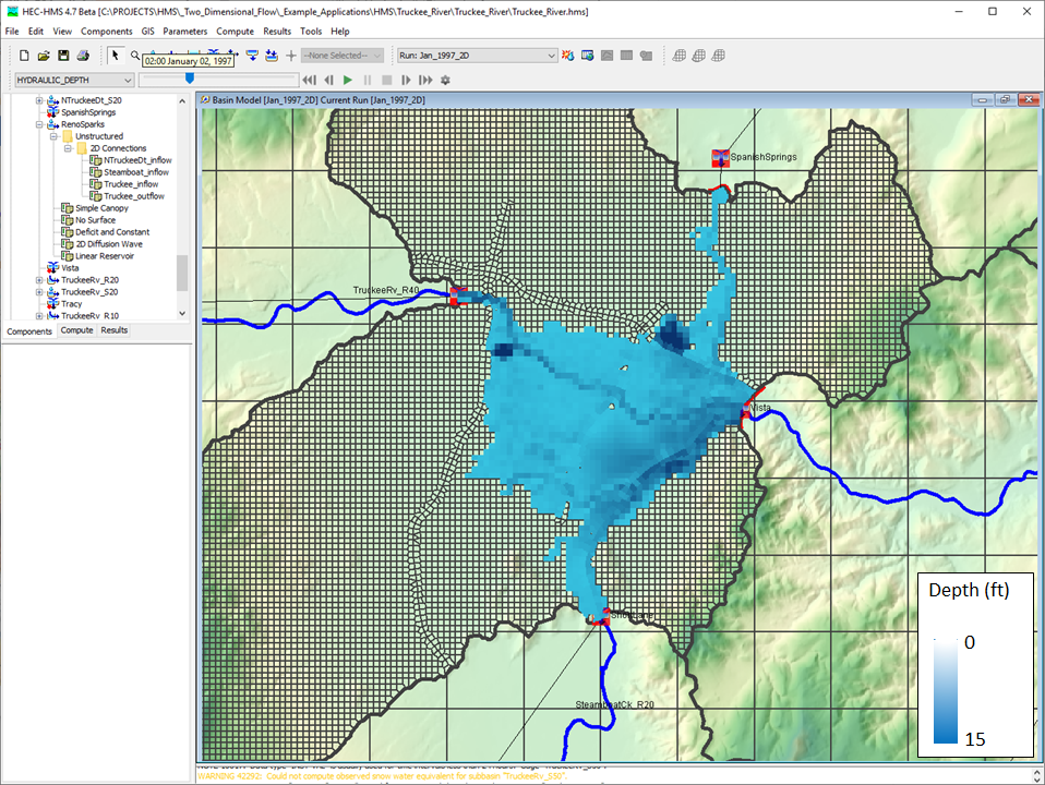
The two-dimensional (2D) flow computational engine that was originally developed for use within HEC-RAS has been made available for use within HEC-HMS as a transform method. This transform method explicitly routes excess precipitation throughout a subbasin element using a combination of the continuity and momentum equations. Unlike unit hydrograph transform methods, this new transform method can be used to simulate the non-linear movement of water throughout a subbasin when exposed to large amounts of excess precipitation (Minshall, 1960). Currently, only the 2D diffusion wave equations can be used within HEC-HMS. This transform method can be combined with all Canopy, Surface, and Loss methods that are currently within HEC-HMS. However, only the None, Linear Reservoir, and Constant Monthly Baseflow methods can be used with this transform method. For instance, the Deficit and Constant Loss method can be used to convert precipitation to excess precipitation, the Simple canopy method can extract infiltrated water through evapotranspiration processes, the 2D Diffusion Wave transform method can be used to route surface flow, and the Linear Reservoir baseflow method can be used to re-introduce infiltrated water as baseflow at the subbasin outlet. Additionally, precipitation that does not initially infiltrate and becomes runoff can infiltrate at a later time or within another grid cell. Spatial variables specific to 2D, such as water surface elevation, hydraulic depth (computed as the volume of water within a cell / wetted area of the cell), and average velocity within a cell, can be displayed within the map. In the following image, hydraulic depth is shown throughout a subbasin that uses the 2D Diffusion Wave transform. Also, videos of hydraulic depth, average cell velocity, and water surface elevation during a flood event are shown below.
Within HEC-HMS, 2D Connections are used to supply boundary conditions as well as link other elements to/from the 2D mesh. Four types of 2D Connections are available for use: Flow, Normal Depth, Rating Curve, and Stage. For instance, if the user wanted to allow flow to leave the 2D mesh using a normal depth assumption, a Normal Depth | 2D Connection could be used. Also, if the user wanted to apply a time series of flow to a 2D mesh, a Flow Hydrograph | 2D Connection could be used. Users must create and link all associated meteorologic boundary conditions (e.g. gridded precipitation, temperature, and/or snow) within HEC-HMS.
The 2D Diffusion Wave transform can only be used with Unstructured or File-Specified Discretizations. As was previously mentioned, an Unstructured Discretization can be created by importing a 2D mesh from an HEC-RAS Unsteady Plan HDF file using the File | Import | HEC-RAS HDF File... option. Unsteady Plan HDF files have extensions of ".p##.hdf" where "p##" corresponds to the specific plan of interest. Currently, users must create a 2D mesh and any associated normal depth, flow, stage, and/or rating curve boundary conditions within HEC-RAS (version 5.0.7 or newer) and then import to HEC-HMS. In the future, users will be able to create and modify both 2D meshes and boundary conditions entirely within HEC-HMS. When importing a 2D mesh from an HEC-RAS Unsteady Plan HDF file, any accompanying boundary conditions for the selected 2D mesh (except for precipitation time series) will be imported and used to create new 2D Connections with the same parameterization. If a File-Specified Discretization is used, the backing file must be in an HDF 5 format and created using either HEC-RAS or HEC-HMS. Pathnames to the HDF file must be limited to a maximum of 256 characters.
Two examples detailing the creation of simple and complex HEC-HMS projects that use the new 2D Diffusion Wave transform can be found here: Creating a Simple 2D Flow Model within HEC-HMS and Creating a Complex 2D Flow model within HEC-HMS. For more see Selecting a Transform Method.
The 2D Diffusion Wave transform capability was funded by the USACE Flood and Coastal R&D program. The project was led by Michael Bartles. Initial code implementation was done by Michael Bartles, Alex Sanchez, and Paul Ely, Contractor. Documentation was done by Michael Bartles. Testing was done by Michael Bartles and Matthew Fleming.
Discretizations
The discretization method defines how a subbasin is discretized. Traditionally, the Mod Clark grid cell file has been used to define the spatially-discrete elements of a subbasin. One limitation of the Mod Clark grid cell file is that it does not use absolute spatial references. Grid cell locations are referenced from an arbitrary lower left corner. Structured and Unstructured discretizations provide spatial-awareness to spatially-discrete subbasin elements. Advantages of the spatially-aware approach include the ability to view discrete elements, the ability to sample values from other geospatial data, and the ability to visualize results for discrete elements.
There are four types of Discretization: Structured, Unstructured, File-Specified, and None.
The Structured Discretization creates a Cartesian grid within the bounds of the subbasin. The Structured Discretization gives options for Standard Hydrologic Grid (SHG) or Universal Transverse Mercator (UTM) projections and 50, 100, 200, 500, 1000, 2000, 5000, or 10000 meter grid cell sizes.
Unstructured Discretizations can have any coordinate reference system and the grid can be unstructured. The backing file format for an Unstructured Discretization is an HDF5 file with identical schema to HEC-RAS, such that files are interoperable. Unstructured grids can be imported from an HEC-RAS Unsteady Plan HDF file (using HEC-RAS version 5.0.7 or newer). The plan file has an extension of ".p##.hdf", where "p##" corresponds to the specific plan of interest. Unstructured grids are most commonly used with the 2D Diffusion Wave transform method.
File-Specified Discretizations were introduced to support the traditional Mod Clark grid cell file, but also support valid Structured Discretization and Unstructured Discretization files. When a File-Specified Discretization is used, the path to a grid-defining file is provided by the user.
The None Discretization represents the entire subbasin as one discrete element within the larger modeling context. This configuration is commonly referred to as a "lumped-parameter." The reality is that all discretization approaches do some amount of spatial-averaging. The amount of spatial-averaging depends on the extent of discrete elements, such as subbasin size or cell size.
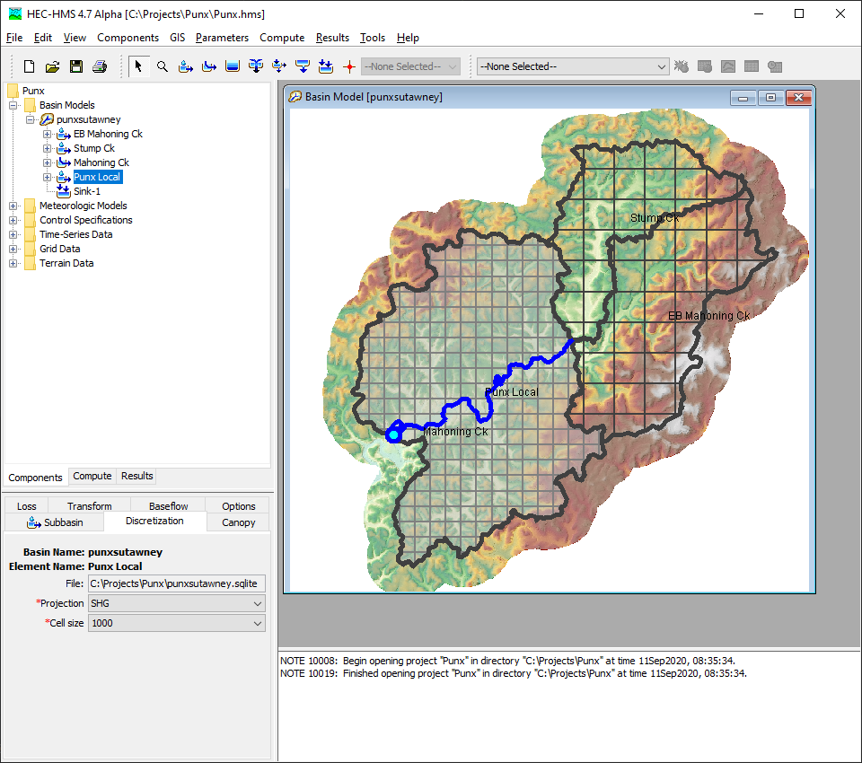
The Punxsutawney basin model shown below uses an SHG projection with 1000 meter grid cell size for the lower subbasin and 2000 meter grid cell size for the upper subbasins.
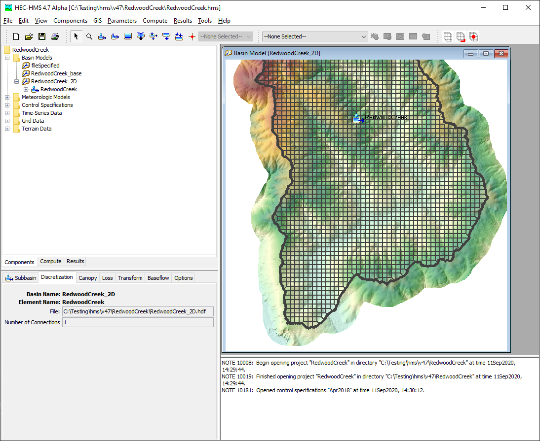
The RedwoodCreek subbasin shown below uses an unstructured discretization.
For more, see Selecting a Discretization Method.
The Discretizations feature was performed as a part of ongoing GIS work. Funding sources include the Flood Control District of Maricopa County, Arizona and the CWMS National Implementation Program. Initial code implementation and documentation were done by Thomas Brauer. Testing was done by Thomas Brauer, Michael Bartles, and Matthew Fleming.
Basin characteristics
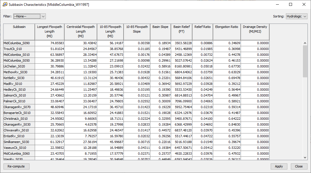
Subbasin and reach characteristics were added to the Parameters | Characteristics menu. To calculate characteristics, the basin model must have spatial features (georeferenced subbasin and reach elements) and flow direction and flow accumulation grids must be calculated. The characteristics are calculated on-the-fly the first time a Characteristics global editor is opened. The characteristics can be re-computed by clicking the button in the lower left of the global editor and the characteristics can be manually edited as well. Characteristics are available as variables in the Expression Calculator. The image below shows subbasin characteristics for the MiddleColumbia_WY1997 basin model.
For more, see Basin Characteristics.
The basin characteristics feature was performed as a part of ongoing GIS work. Funding sources include the Flood Control District of Maricopa County, Arizona and the CWMS National Implementation Program. Initial code implementation and documentation were done by Thomas Brauer and Josh Willis, USACE Ft. Worth District. Testing was done by Thomas Brauer, Josh Willis, Michael Bartles, and Matthew Fleming.
Expanded ASCII/GeoTIFF grid support
The grid management framework was updated in v.4.6 to accommodate ASCII format precipitation-frequency grids. In this release, all parameter grids were updated to accept ASCII and GeoTIFF data sources in addition to the HEC-DSS format. The ASCII and GeoTIFF options were not added to gridsets, or time-series of grids, like precipitation and temperature gridsets. ASCII and GeoTIFF parameter grids can be sampled in the new Expression Calculator.
The image below shows a GeoTIFF percolation parameter grid selected in the component editor.
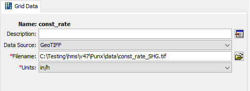
For more information, seethe Grid Data and Parameter Estimation sections in the User's Manual. The expression calculator has only been implemented for a few subbasin methods.
The expanded parameter grid feature was performed as a part of ongoing GIS work. Funding sources include the Flood Control District of Maricopa County, Arizona and the CWMS National Implementation Program. Initial code implementation and documentation were done by Thomas Brauer. Testing was done by Thomas Brauer, Michael Bartles, and Matthew Fleming.
GIS parameter estimation
An Expression Calculator has been added to facilitate parameter estimation from GIS data. The Expression Calculator can be launched from select global basin editors. This release includes an initial implementation for Deficit and Constant and Green and Ampt loss and Mod Clark, Clark, and S-Graph transform global editors. The expression calculator requires the basin model to have spatial features (georeferenced subbasin elements). In the Expression Calculator, grids and characteristics and can be used as variables. When a grid is included in the expression, a zonal average value for the feature-grid combination is used in the calculation. When a characteristic is used in the expression, the characteristic value for the feature (subbasin element) is used in the calculation.
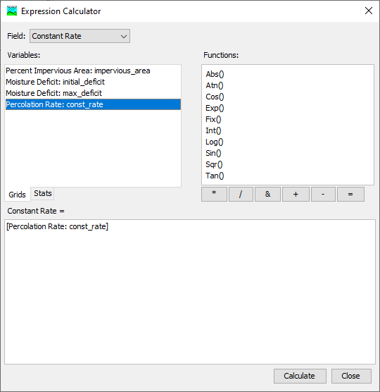
In the image below, a Parameter Grid has been included the expression. The program will compute the average value per subbasin (using a zonal average GIS function) and populate the constant loss rate parameter for all subbasins.
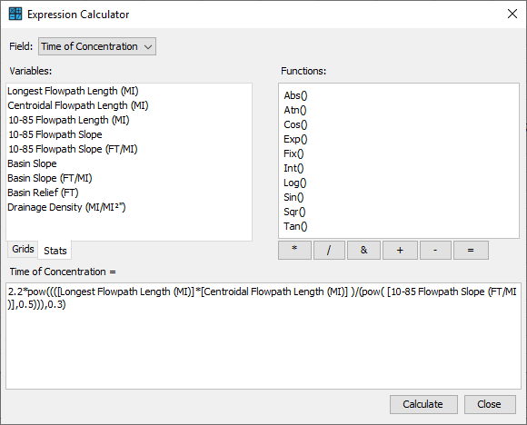
In the image below, the subbasin characteristics (longest flowpath, centroidal flowpath, and flowpath slope) have been included in the expression to compute the time of concentration for each subbasin.
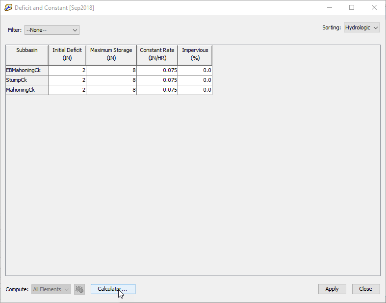
The Expression Calculator is launched from the Calculator... button at the bottom of a global editor.
For more, see Parameter Estimation
The expression calculator feature was performed as a part of ongoing GIS work. Funding sources include the Flood Control District of Maricopa County, Arizona and the CWMS National Implementation Program. Initial code implementation was done by Thomas Brauer and Nick Van. Documentation was done by Thomas Brauer. Testing was done by Thomas Brauer, Michael Bartles, and Matthew Fleming.
Gridded Data Import Wizard
A new utility Gridded Data Import Wizard has been added to HEC-HMS to convert supported data formats, e.g. NetCDF, GRIB, HDF, and ASC, to the HEC-DSS format. The utility is based on the Vortex Importer utility. The Import Wizard can be launched from the HEC-HMS File | Import | Gridded Data menu.
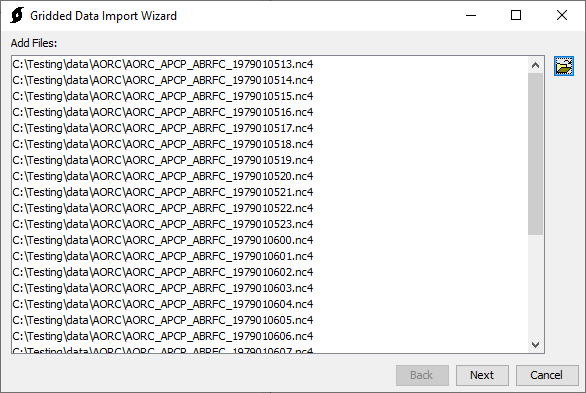
For more information, see Gridded Data Import Wizard.
The Vortex R&D project has been funded by the USACE General Investigations program. Thomas Brauer has been principal investigator for the project. Nick Van performed the Gridded Data Importer Wizard user interface implementation for HEC-HMS.
Spatial results visualization
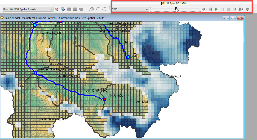
A new capability to visualize computed results has been added to HEC-HMS. The following figure shows the Spatial Results toolbar along with SWE results displayed on top of the basin model. The Spatial Results toolbar includes options for selecting output results, an animation toolbar, buttons for controlling the animation, and an Animation Setting button that opens an editor with options for color ramps, scale, animation speed, and whether the animation should loop. Spatial results will only be available for simulations that have basin models with georeferenced subbasin elements. A georeferenced basin model is one where either the subbasins and reaches were delineated using the GIS tools, or one where subbasin elements were georeferenced using a shapefile (Georeference Existing Elements or Import Georeferenced Elements). Gridded spatial results cannot be visualized for subbasin elements using the ModClark file option (under the Specified File discretization method). Instead, results will be displayed as a subbasin average value when the *.mod file option is used. Gridded spatial results can be visualized for the structured, unstructured, and File-Specified *.sqlite, *.HDF5, and *.HDF discretization options.
Spatial results can be displayed for both simulation runs and forecast alternatives. Spatial results must be activated in the simulation's Component Editor, as shown below. There is an option to choose the time interval for the spatial results. By default, the time interval is the simulation run time step; however, a larger interval can be selected to reduce the amount of output. Spatial results are saved to an HDF5 file within the project's "results" directory. The very first time an output result is selected in the Spatial Results toolbar, the program will process the simulation HDF5 and build animation tiles for display. The animation can be controlled through the animation toolbar, and the visual properties of the results can be changed as well.
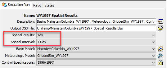
For more see Viewing Spatial Results.
The spatial results feature was funded by the the USACE Flood and Coastal R&D program. The project was managed by Thomas Brauer. Initial code implementation was performed by Caleb Dechant, Contractor, and Paul Ely, Contractor. Documentation was done by Matthew Fleming. Testing was done by Thomas Brauer, Michael Bartles, and Matthew Fleming.
Bug Fixes
Reservoir storage is incorrect when using FT:FT2 or M:M2 elevation-area function
This bug was incorrectly reported as fixed in v.4.4. Storage volumes and discharge were incorrect due to an incorrect unit conversion when using FT:FT2 or M:M2 as an elevation-area function in the reservoir routing method.
Gridded Green and Ampt: Incorrect parameterization in the component editor
The Green and Ampt Loss Component Editor has two options for the initial soil moisture, Initial Deficit and Initial Content. The user must select Initial Content and Saturated Content grids when the Initial Content option is selected. The user must select an Initial Deficit grid when the Initial Deficit option is selected. There was a bug where the program required a Saturated Content grid when the Initial Deficit option was selected. Now, the program no longer requires the user to specify a Saturated Content grid when the Initial Deficit option is selected.
Standard Report: Incorrect Units Displayed
In the report generated by the Standard Report option, the system of units (U.S Customary or Metric) used in the basin model was not reflected in the "Global Results Summary" section of the report. Previously, only U.S Customary units were used regardless of the system of units. The bug has been fixed such that data reported is consistent with the system of units used in the basin model.
Beta releases
Initial beta released
- Updated spatial results: better handling for lumped vs gridded methods, default color ramps and scales set per variable, and control over output write interval. Added indexed value mapper for roughness grid. Added re-indexing logic for gridded precipitation on lumped subbasin with structured discretization. Migrated linear reservoir baseflow editor to new framework. 2D flow capabilities: added default color ramps and scales for 2D flow spatial variables (depth, MMC depth, water surface elevation, and cell velocity), bugfixes and updates to the 2D Connection component editor.
Features: Added met data import wizard. Added new global editor framework for linear reservoir baseflow, Clark UH, Green & Ampt, user-specified S-graph. Added additional characteristics/units to "stats" tab of Expression Calculator. Added ASCII/GeoTIFF option for all static grid types. 2D bugfixes/features branch merged. Bugfixes: Force recompute meteorology if discretization changes. Re-index grid cells when gridded precipitation is used with non-gridded subbasin. Recompute simulation if spatial results interval changes. Avoid subsetting raster during sampling when raster is already clipped to subbasin. Initialize Global Basin Editor and Global Characteristics View to hydrologic order. Use the correct S-graph lag parameter when the Maricopa/regression approach is used. Correctly adjust reservoir area provided as meters squared to thousand meters squared. 2D bugfixes/features branch merged. 2D flow capabilities: added cumulative outflow and stage time series, bugfixes, and updates to the 2D Connection component editor.
- Added Gridded Data import option from the File | Import menu. The Gridded Data import option was adapted from the HEC-Vortex Importer utility. 2D flow capabilities: improved visualization of downstream connections for 2D Connections, fixed 2D spatial results bugs, and added error checks when importing a 2D mesh from HEC-RAS. Fixed a bug where reports generated by the Standard Report option only displayed US Customary units in 'Global Results Summary' section.
- Added Expression Calculator Precision setting to Tools | Program Settings, Compute tab. Added handling logic for the case where a discretization geometry calculation is attempted and there is no flow direction grid. 2D flow capabilities: fixed a bug that incorrectly removed the downstream connection when saving a 2D mesh and improved error checking prior to a compute. Fixed a bug within the Initial Deficit grid selection when using the Gridded Green-Ampt loss method. Added logic to allow for more intuitive interaction with the spatial results animation tool bar.
General Acknowledgments
Many engineers, computer specialists, and student interns have contributed to the success of this project. Each one has made valuable contributions that enhance the overall success of the program. Nevertheless, the completion of this version of the program was overseen by Matthew Fleming while Christopher N. Dunn was Director of the Hydrologic Engineering Center. Thomas Brauer led the HEC-HMS team during the Version 4.7 release cycle. HEC-HMS team members include Thomas Brauer, Michael Bartles, David Ho, Gregory Karlovits, Jang (Jay) Pak, Alejandro Sanchez, Nick Van, and Josh Willis.