Advanced Inline Structure Modeling - Example 18

This example will demonstrate the use of HEC-RAS to analyze a river reach that contains an inline structure that features a weir, gated spillway, culverts, outlet rating curve, and inline time series outlet. Emphasis is given to demonstrating how to utilize the Inline Culvert, Outlet RC, and Outlet TS functions.

To perform the analysis the user must enter the geometric data for the various inline structure components along with the geometry of the river reach. Then, the user must enter the rating curve for the Outlet RC function, a flow hydrograph for the Outlet TS, and a time series gate opening for the gated spillway. The flow hydrograph and the time series gate opening are entered as internal boundary conditions in the Unsteady Flow Editor. The modeler is referred to Chapter 6 of the User's Manual for discussion on entering the geometric data for the weir, culverts, and gated spillway; Chapter 8 of the User's Manual for entering the gate opening flow data; Chapter 6 of the Hydraulic Reference Manual for the hydraulic analysis procedures for analyzing the flow through the culverts; and Chapter 8 of the Hydraulic Reference Manual for the hydraulic analysis procedures for analyzing the flow through the gate openings and over the weir.

To review the data files for this example, from the main HEC-RAS window, select File and then Open Project. Go to the directory in which you have installed the HEC-RAS example data sets. From the "Applications Guide\Example 18 – Advanced Inline Structure" subdirectory, select the project labeled "Advanced Inline Structure Example." This will open the project and activate the following files:

Plan: "Unsteady Flow – Inline Structure"
Geometry: "Beaver Cr. – Adv Inline Structure"
Flow: "Unsteady Flow Data"

Example 18 - Advanced Inline Structure.zip

Geometric Data

To view the geometric data for the river system, from the main program window select Edit and then Geometric Data. This will activate the Geometric Data Editor and display the river system schematic as shown in the figure below. The schematic displays the 59 river stations of the reach "Kentwood" on "Beaver Creek", with river station 5.99 as the upstream cross section and 5.0 as the downstream cross section. In addition to the inline structure, the river reach has a lateral structure that is connected to a storage area. For further information on modeling lateral structures connected to a storage area see "Unsteady Flow Application – Example 17."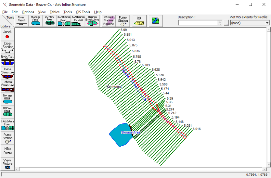

Cross Section Data

The cross section data consists of the X-Y coordinates, Manning's n values, contraction and expansion coefficients, etc. The user can view this data for each river station by selecting the Cross Section icon on the left side of the Geometric Data Editor. For this example, an inline structure was added at river station 5.26 and will be discussed in the next section.

Cross Section Placement

The placement of the cross sections in reference to the inline structure should be treated much like that for bridges and culverts. The flow will contract to enter the various inline structure openings and expand after exiting the openings. The program will use four cross sections located on both sides of the structure to define the contraction and expansion of the flow through the structure. To provide guidance for the expansion reach length and contraction reach length, the tables in Appendix B of the Hydraulic Reference Manual were utilized. These tables were developed based on data for flow through bridges; however, they were used to provide general guidance. For further guidance on cross section placement for inline structures look to "Inline Structure - Example 12" as well as Chapter 6 of the User's Manual.

Ineffective Flow Areas

As performed for bridges and culverts, ineffective flow areas should be entered on the cross sections that bound the inline structure. For this example, the cross section that is upstream of the structure is 5.274 and the cross section downstream of the structure is 5.258. For further information on placing ineffective flow areas for inline structures see "Inline Structure - Example 12" as well as Chapter 6 of the User's Manual.

Inline Structure

To add an inline structure, the Inline Structure icon was selected from the left side of the Geometric Data Editor. This activated the Inline Structure Data Editor as shown in the figure below. Next, Options and Add an Inline Structure were selected and river station 5.26 was entered as the location for the inline structure. The schematic then displayed the cross section data for the river station immediately upstream of the inline structure location: namely river station 5.274 for this example.

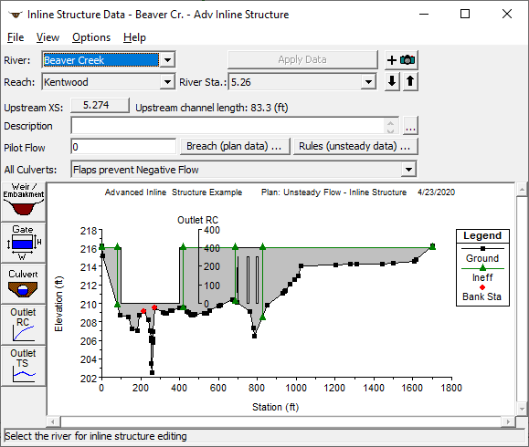
Since there are no flap gates on the culverts, No Flap Gates was selected from the All Culverts dropdown menu in the center of the Inline Structure Data Editor. "Flaps prevent Negative Flow" can be selected in cases where flap gates prevent the inline structure's tailwater from propagating upstream through the culverts. (e.g. Immediately downstream of the inline structure the river empties into a bay whose tidal fluctuations are impeded at the culverts by flap gates.) "Flaps prevent Positive Flow" prevents the culverts from passing flow from upstream to downstream; however, flow can pass from downstream to upstream.

Weir/Embankment

To enter the data for the weir, the Weir/Embankment icon was selected from the left side of the Inline Structure Data Editor. This activated the Inline Structure Weir Station Elevation Editor as shown in the figure below. This editor is similar to the deck/roadway editor used for bridges and culverts. Further insight and instruction on the Weir/Embankment function can be found in "Inline Structure – Example 12" and Chapter 6 of the User's Manual.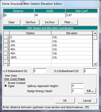

Gated Spillways

To enter the data for the gates, the Gate icon was selected from the Inline Structure Data Editor (second figure on this page). This activated the Inline Gate Editor as shown in the figure below. For this example, one sluice gate was entered.

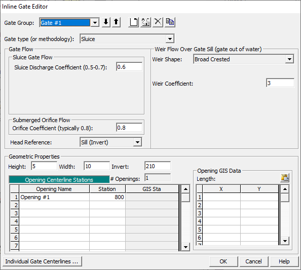
When the Inline Gate Editor was activated, the first gate was automatically labeled as "Gate #1." The Height, Width, and Invert for the gate were entered as 5, 10, and 210 feet, respectively. On the lower left side of the editor, the centerline station for the gate was entered as shown in the figure above. The # Openings automatically updates to coincide with the number of centerline stations entered. In this case there is only one opening.

The remaining portion of the editor is divided into two sections, one for the Gate Flow data and one for Weir Flow data. For the gate data, the first field is the Gate Type. For this example the gate type was left at the default type "Sluice". The Sluice Discharge Coefficient was entered as 0.6, while the default value of 0.8 was used for the Orifice Coefficient. The orifice coefficient is only used for fully submerged flow conditions. Additionally, the head reference for the gate equation defaults to the "Sill (invert)" of the gate opening.

For the Weir Flow data, the Weir Shape was kept at the default shape of "Broad Crested" and the Weir Coefficient was kept at the default value of three.

The OK button was selected at the bottom of the Gate Editor and the gate appeared on the Inline Structure Data Editor as shown in the second figure on this page. (Note: The ineffective flow areas will be entered after entering all the geometric data for the inline structure components.) At this point, the user should zoom in on the gate opening to ensure that they do not overlap with other features and appear as intended. The Inline Structure Data Editor was then closed.

Culverts

To enter the data for the culverts, the Culvert icon was selected from the Inline Structure Data Editor (second figure on this page). This activated the Culvert Data Editor as shown in the figure below. The Culvert Data Editor for the inline structure is identical to the one used under the Bridge/Culvert icon found in the Geometric Data Editor. In this example two culverts were used, one circular culvert and one box culvert. For more information on entering culvert data refer to "Single Culvert (Multiple Identical Barrels) Example 3" and "Multiple Culverts Example 4".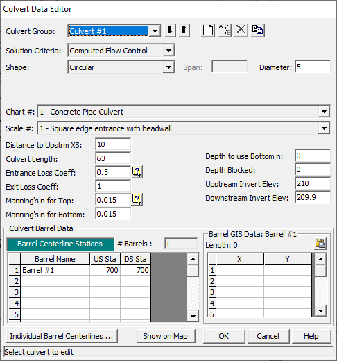

Outlet Rating Curve

Next, the Outlet RC icon was selected. The Outlet RC feature allows the user to account for inline structure discharges that can't be properly modeled by the weir, gate, or culvert features.

Once the Outlet RC icon was selected, a window appeared that provided a table to enter the rating curve information (below). The radio button Outlet flow based on water surface upstream was selected to signify that the relationship between the diversion flows from the structure has a direct correlation to the upstream water surface elevation. If the diversion flow was instead based on the upstream flow rates then the Outlet flow based on flow upstream radio button would be selected, causing the heading of the first column of the table to change from US WS Elev to US Flow.

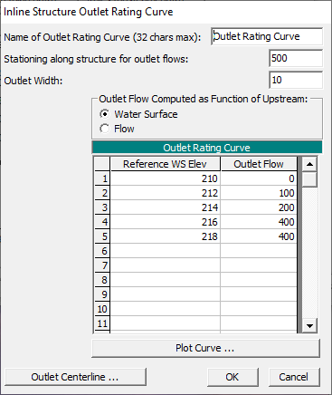
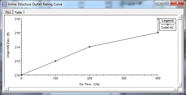
The outlet rating curve table was filled in with the values seen in the figure above. It should be noted that if the calculated water surface elevation is outside the upper or lower bounds of the rating curve the program uses the two nearest points on the rating curve to linearly extrapolate a diversion flow value to correspond to the calculated water surface elevation. Once the values are entered in the table, the resulting rating curve can be plotted and graphically inspected by clicking Plot Curve. The outlet's rating curve is plotted in a separate window as seen in the figure below. After filling in the table and viewing the plot, click the OK button in the lower right hand corner of the Inline Structure Outlet Rating Curve window.

Time Series Outlet

Time series outlets are used to account for time dependent flow releases that take place at the inline structure. Often times, as with this example, this feature is used to model the flow going through a hydropower facility adjacent to the inline structure.

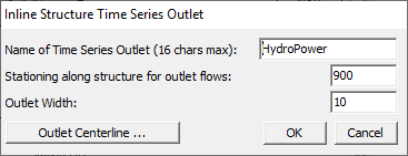
First, the Outlet TS icon from the Inline Structure Data Editor (second figure on this page) was selected to signify that a time series outlet exist at the specified location. This activated the Inline Structure Time Series Outlet window as shown in the figure below. The name given to the time series outlet was "HydroPower". After naming the outlet, press OK.

The time series outlet is time dependent; therefore, the operation of the outlet is event specific and cannot be entered in as geometric data like the other inline features. Instead, a flow hydrograph is created at the inline structure cross section as an internal boundary condition in the Unsteady Flow Editor. The name given to the time series outlet (i.e. "HydroPower") is not seen on the Unsteady Flow Editor; however, the title does appear on the various output tables once the model is computed. How to enter the flow hydrograph in the Unsteady Flow Editor will be explained further in the next section.

Unsteady Flow Data

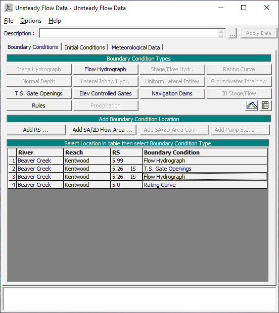
The user is required to enter boundary conditions and initial conditions for the system at the beginning of the simulation period. For additional information on unsteady flow data refer to Chapter 8 of the User's Manual, Performing an Unsteady Flow Analysis. The Unsteady Flow Data Editor, shown in the figure below, was selected from the main program window under the Edit menu.

Boundary Conditions

Boundary conditions are required for the farthest upstream and downstream cross sections. Upon entering the Unsteady Flow Data Editor the farthest upstream and downstream cross sections will be located in the boundary conditions column. In this case, the user will see River Station 5.99 and River Station 5.0 as the upstream and downstream boundary conditions, respectively. Boundary conditions are set by highlighting the adjacent cell under Boundary Condition Type. When a cell is highlighted, not all boundary conditions are available. The program will automatically gray out all irrelevant boundary condition types. Internal boundary conditions may be added by selecting one of the buttons under the "Add Boundary Condition Location" heading.

Upstream Boundary Condition

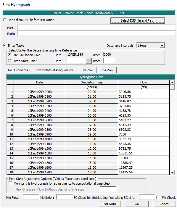
For River Station 5.99 a flow hydrograph was selected by highlighting the cell and pressing the Flow Hydrograph button. The window for a Flow Hydrograph is shown in the figure below. The user may select to read hydrograph data from a DSS file or manually enter the data. For further instruction on using a DSS file see Unsteady Flow Application Example 17. For this example the flow hydrograph was manually entered by selecting the Enter Table radio button. The Data Time Interval was set to one hour and the radio button Use Simulation Time was selected causing the initial propagation of the hydrograph to coincide with the beginning of the simulation time window. The hydrograph was then manually entered into the table.

Downstream Boundary Condition

For River Station 5.0 the boundary condition selected was a rating curve. Again, the corresponding cell for that particular river station was highlighted and the Rating Curve button was selected. The window shown in the figure below is then displayed and the user is given a choice whether to Read from DSS before simulation or Enter Table. For this example the Enter Table radio button was selected and the stage and flow values were entered in the appropriate units.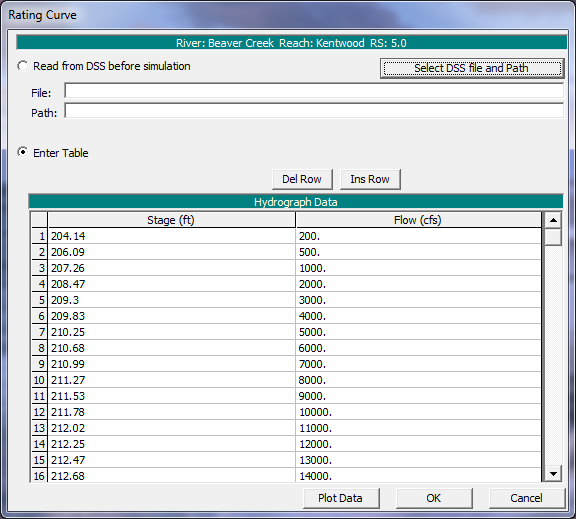

Internal Boundary Conditions

Two internal boundary conditions were entered at River Station 5.26 for the gate and Outlet TS (titled "HydroPower" in this example) of the inline structure. A new boundary condition was entered by selecting Add RS from the Unsteady Flow Data window, and specifying the desired river station location (5.26). Once the desired river station was selected and appeared in the Selected Locations box, the OK button was clicked. The River Station 5.26 was populated in the Boundary Conditions Table. The "IS" that appears next to River Station 5.26 signifies that there is an inline structure at that location. The corresponding cell next to River Station 5.26 was highlighted under the Boundary Condition column and the T.S. Gate Openings button was selected for the first internal boundary condition.

Upon selecting T.S. Gate Openings as the boundary condition a window opens up titled "Gate Openings". The radio button Enter Table was selected. The Data time interval dropdown was kept at the default of 1 Hour. Under Select/Enter the Data's Starting Time Reference the Use Simulation Time radio button was selected, automatically filling in the Date and Time fields. The only remaining field to be populated was the Gate Opening Height. In this example the gate height remained constant at five feet (see figure below). Once all the data was entered, the window was closed and the data was stored by clicking OK.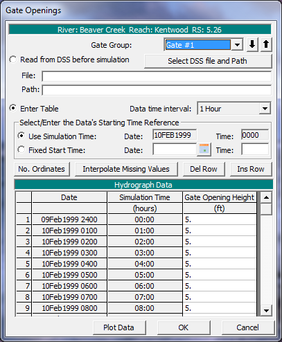

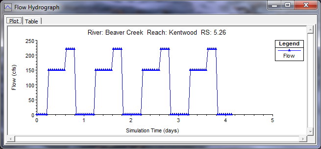
Next, the corresponding cell for the other internal boundary condition (also at RS 5.26 IS) was highlighted under the Boundary Condition column. The Flow Hydrograph was chosen to represent the time series outlet titled "HydroPower". The Flow Hydrograph data entry window that appears has the same inputs as the T.S. Gate Openings boundary condition just completed. The same parameters were entered for both with the exception of the flow values under the Flow column under the Hydrograph Data table. Since the hydrograph represents the flow of a hydroelectric facility, there is some daily variability in the flows (as seen in the figure below). In this example, there is zero flow during the hydro facility's non-peak hours (8 p.m. – 6 a.m.), 150 cfs flow from 6 a.m. – 3 p.m., and during peak energy demand hours (3 p.m. – 8 p.m.) there is 220 cfs diverted through the hydropower facility. Once all the data was entered, the window was closed and the data was stored by clicking OK.

Initial Conditions

Initial conditions consist of flow and stage information at each of the specified cross sections, as well as elevations for any storage areas defined in the system. Data for initial conditions is established by selecting the Initial Conditions tab on the Unsteady Flow Data Editor. After selecting the tab, the figure below will be displayed.

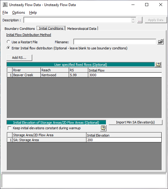
As seen in the figure above, the Enter Initial flow distribution radio button was selected and an initial flow of 3000 was entered for the most upstream river station (5.99). In addition to flow data, the initial elevation for the storage area is needed. The initial elevation of the storage area was set to 200. The data was then saved (File -> Save Unsteady Flow Data As…) in the Unsteady Flow Data Editor and the window was closed.

Unsteady Flow Analysis

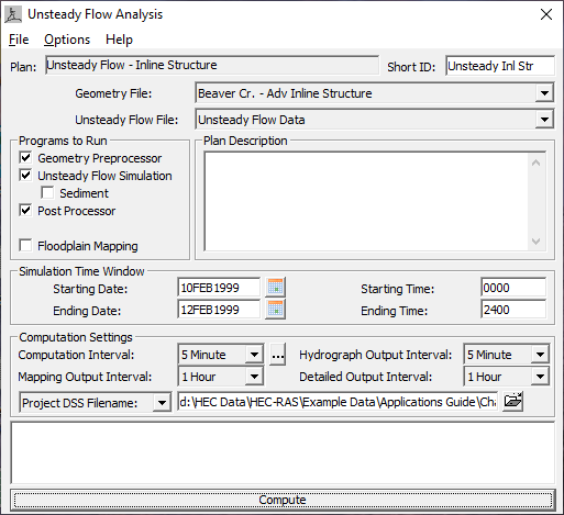
After the geometry and unsteady flow data have been completed an unsteady flow analysis may be initiated. Under the main program window Unsteady Flow Analysis was selected under the Run menu; this displayed the Unsteady Flow Analysis Window shown in the figure below. A plan was defined by selecting the Geometry File "Beaver Cr. – Adv Inline Strc" and the Unsteady Flow File "Unsteady Flow." Under the File menu, Save Plan As was selected and the plan title was entered as "Unsteady Flow - Inline." After entering the title of the plan a short identifier was entered as "Unsteady Inline" and the plan was saved. For more information on the Simulation Time Window, Computation Settings, and Location of Stage and Flow Hydrographs (Under Options) refer to "Unsteady Flow Application – Example 17".

Output Analysis

For the analysis of the output, the water surface profiles, the inline structure type cross section table, and the inline structure type profile table will be reviewed. Each of these is discussed in the following sections.

Water Surface Profiles

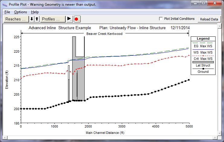
The water surface profiles are shown in the figure below. This figure was activated from the main program window by selecting View and then Water Surface Profiles. The figure shows the maximum water surface elevation. The entire event can be seen as an animation by selecting Options and then Animate from the profile plot window.

Inline Structure Detailed Output Table

To review the flow parameters through the inline structure components, the Inline Structure type Detailed Output Table is activated. This table was activated from the main program window by selecting View, Detailed Output Table, Type, and then Inline Structure.

At the top of the table, the profile "Max WS" was selected. The table itself is broken into two columns. The first column lists the energy grade and water surface elevations, a summary of all discharges from the inline structure, and breach information (not applicable in this example). The second column gives more detail on the performance of the weir and gate structures. The Inline Structure Output table can be seen in the figure below.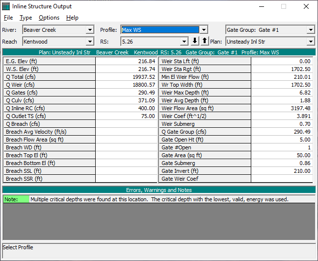

Inline Structure Profile Summary Table

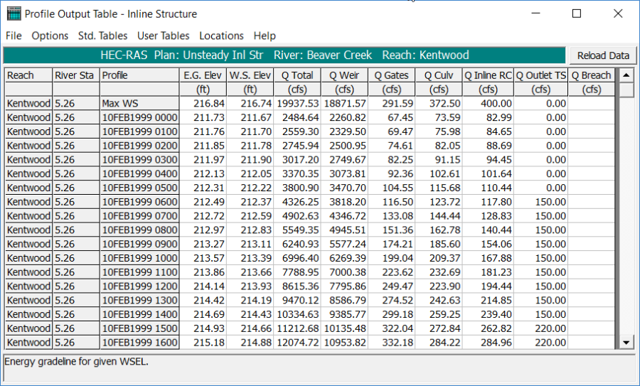
Finally, the Inline Structure Profile Summary Table is shown in the figure below. This figure was activated from the main program window by selecting View, Profile Summary Table, Std. Tables, and then Inline Structure. The figure displays the water surface elevations, energy grade line, and total weir and gate flows for each of the profiles. The advantage of this table over the Inline Structure Detailed Output Table is that the user can compare all the profiles at the same time.

Summary

This example computed an unsteady flow event through a complex inline structure on Beaver Creek, which included an inline weir, culverts, gated spillway, outlet rating curve, and a time series outlet. The example demonstrated how to make use of the various inline features noted above.

In addition, a brief overview was given on the output profiles and tables that can be utilized in evaluating the operation of the inline structure. The output tables and profiles described were the Inline Structure Output table, Profile Summary Output Table - Inline Structure, and Profile Plot.