Download PDF
Download page Introduction to Regional Precipitation Frequency Analysis Using R Workshop.
Introduction to Regional Precipitation Frequency Analysis Using R Workshop
If at any time you need a refresher on working with R commands or on how to use RStudio, feel free to look back at the R Introduction or the RStudio introduction pages.
Workshop Files
Download the workshop files here. To avoid issues with broken links in the R Project, do not unzip the project in deeply nested folders. Instead, download it to a simple, high-level directory (e.g., C:/Projects/). Long pathnames can cause problems! Regional_Precip_Frequency_Workshop.zip
This is a two-part workshop that introduces the principles and application of regional precipitation frequency analysis (RFA) using R. RFA is a statistical technique that improves the reliability of frequency estimates by pooling data from multiple stations that share similar climatic and hydrologic characteristics. By leveraging the method of L-moments, RFA allows for more stable estimates, especially in regions with short or missing data records.
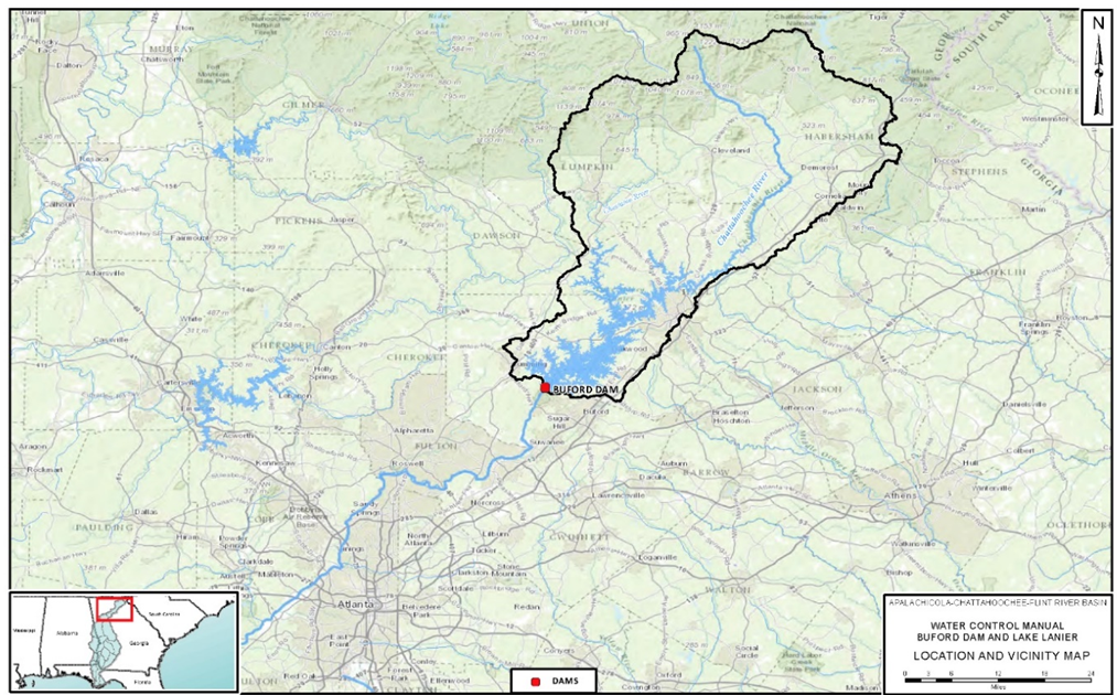
This workshop focuses on Buford Dam, located approximately 35 miles northeast of Atlanta, Georgia. Buford Dam is a key reservoir and flood control structure in the southeastern U.S., making it an important location for analyzing extreme precipitation events and understanding regional patterns.
Disclaimer: The United States Army Corps of Engineers has granted access to these data for instructional purposes only. Do not copy, forward, or release the information without United States Army Corps of Engineers approval.
Project Structure
To keep everything organized and reproducible, this workshop uses an R Project folder structure. When you open the project in RStudio, you will see:
Two
.RmdNotebooks, one for each taskA
data/folder for both input data and saved outputsA
helper/folder, which contains a special tool: at certain points in the workshop, you will be prompted to type something into the console to receive hints or answers- A
renv/folder, which performs package management and ensures that all necessary R packages are installed and the same versions are used by everyone - A
solutions/folder that contains the solutions of each Notebook
Once you open the R Project, you can click on either "task1_data.Rmd" or "task2_regional_frequency_analysis.Rmd" to begin the task. You do not need to go into any of the folders, and you do not need to install any packages as these are already included in the R Project thanks to renv. It is recommended to view the R Notebooks in "Visual" mode rather than "Source" mode (you can switch modes using the button in the upper-left of the editor tab). Visual mode makes it easier to read, write, and run code chunks in R Notebooks, especially if you're new to R.
Finally, As you work through the notebooks, you can run individual code chunks by clicking the "Play" button next to each one. If you'd like to see a full output or save the Notebook as a viewable PDF or HTML, use the "Preview" or "Knit" button at the top of the editor to generate a clean report that includes both code and output. These features help you check your progress and review your results in a readable format.
For more information on these features in R, please check these links:

Tasks
The workshop is structured into two tasks:
Task 1: Data Preparation
In this first task, we’ll build the foundation for the analysis by preparing the Annual Maximum Series (AMS) from daily precipitation records. Using data from the Global Historical Climatology Network (GHCN), we will select gages within our study area, download data and perform quality control, and extract annual maxima from each station to construct the AMS. This cleaned and standardized dataset will be used in the second task.
Task 2: Regional Frequency Analysis
Building on the AMS data, the second task focuses on applying regional frequency analysis using the method of L-moments. We will visualize and explore the study area and precipitation data that we collected. We will then apply the procedures as outlined in Hosking & Wallis (1997) with support from the lmom and lmomRFA R packages. By the end of the workshop, we will have completed most steps in a typical regional frequency analysis.
Continue to Task 1: Data
