Sampling Forecast Uncertainty
The Hydrologic Sampler's Bootstrap Sampling method allows the sampling of forecasts, such as those used to determine reservoir draft requirements in watersheds with snowmelt-dominated or otherwise seasonal hydrology. Sampling forecasts requires entering an observed volume and accompanying statistical parameters of the forecast error term, also known as forecast skill.
If sampling of forecast uncertainty is required, enable the feature by checking the Include Forecasts checkbox at the top of the Hydrologic Sampling Editor (review Selecting Bootstrapping Historical/Synthetic Basin-wide Events method). This will allow entry of the required forecast locations, associated skill parameters, and observed values to sample forecast error around.
Under the initial Settings tab, in the Forecasts tab, users will define forecast locations from among flow locations that have already been defined. From the Forecast Statistics panel, a table for entering the forecast statistics for each defined forecast location is available. The Edit Spatial Correlation button opens the Edit Forecast Correlation dialog containing a spatial correlation table (review the Spatial Correlation section).

It is important to note that users can only generate random hydrologic forecasts for flow at locations already defined in the watershed. In other words, forecast locations can only be selected from the list of available locations, and only those for which flow is specified as a parameter. For this reason, the Locations & Parameters tab must have at least one location selected with flow as a specified parameter before the Forecasts tab can be completed. If a hydrograph location has not been selected and assigned flow and users attempt to add forecast locations, then a No Available Locations message window will open, reminding the user to first define hydrograph locations (primary locations) before trying to select forecast locations. Therefore, the hydrograph location setup must be completed (review Hydrograph Locations and Parameters) prior to including forecast locations in a hydrologic sampling alternative.
Select Forecast Locations
Forecast Locations are the Common Computation Points where the Hydrologic Sampler should generate sampled forecasts. These are often a subset of the inflow locations used by the model.
The first step is to select forecast locations from the defined hydrograph locations of the watershed:
- From the Forecasts tab, click Select Forecast Locations, a Selection Editor will open. The editor allows users to identify forecast location(s) from the list of hydrograph locations that have been defined for the watershed with flow as a parameter (e.g., Dworshak_IN).
- Select forecast location(s) from the Available Locations list individually, or select multiple locations while holding down the Ctrl key, click Add, this will move the selected location(s) to the Selected Locations list. Add All moves all locations from the Available Locations list to the Selected Locations list. Alternatively, double-clicking on a desired location (e.g., Hilldale) will move the location form the Available Locations list to the Selected Locations list.
To remove locations from the Selected Locations list, select a location, either click Remove for individually selected locations, or click Remove All to remove all selected locations from the Selected Locations list, and move the locations back to the Available Locations list.

Note
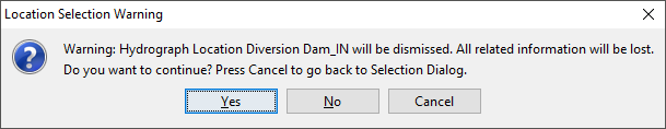
Users can add or remove forecast locations at any time. However, if users attempt to remove forecast locations, a Location Selection Warning message window will open, which requires users to confirm the deletion of the selected forecast location(s) and all related information.
- Following the successful selection of the forecast location(s), click OK, and the Selection Editor will close.
- The Location list will now contain the selected forecast locations. For each forecast location, the user will need to define forecast statistics.
Forecast Statistics
Once the forecast location(s) have been defined, users need to complete the forecast statistics table for each date at which a new forecast should be issued. Information required for the table includes forecast dates and error statistics for each identified forecast location. The error statistics of mean, standard error, serial correlation and spatial correlation are used in the AR(1) forecast generation process. At least one forecast date (e.g., 01Jan) needs to be defined for a forecast location.
Define the forecast date(s), forecast statistics, and serial correlation for each forecast location:
- From the Location list, select a forecast location of interest (e.g., Dworshak_IN).
- In the Forecast Statistics table, from the Date column, click the dropdown list to select a forecast date (e.g., 01Jan).
- The Min Forecast Override value is used to prevent a minimum forecast below a reasonable value from being generated. The user should enter the smallest reasonable forecast value (kilo-acre-feet, KAF) that can be produced by the real-time forecast method (e.g., 947.14) that would be produced in real-time decision-making. This value can be derived directly from historical forecast data.
- Forecasts tend to be biased toward the average of possible outcomes of the value being forecasted, known as the central tendency of the forecasting process. Thus, large volumes tend to be under-forecasted, and small volumes tend to be over-forecasted. The Hydrologic Sampler random forecast generation method uses a bias line that defines a mean forecast error as a function of the starting forecast value. The mean forecast error for a given observed volume is used by the autoregressive lag 1, AR(1), forecast generation. The Relationship of Error to Magnitude data provides the necessary data for representing the central tendency term:
- From the Mean Error Intercept column, the user will enter the intercept of the error bias line (e.g., 863.5148) in KAF. Enter 0.0 if no bias line is desired.
- From the Mean Error Slope column, the user will enter the intercept of the slope of the error bias line (e.g., -0.32922). Enter 0.0 if no bias line is desired.
From the Standard Error column, the user will enter the standard error that will be used in the AR(1) forecast generation (e.g., 419.52204). This standard error represents the width of the distribution of forecast errors around the central tendency mean.
Because of the central tendency term, this Standard Error is not the same as the root mean square error (RMSE) of the forecast.
- When more than one forecast date has been entered in the forecast statistics table, a serial correlation of forecast must be defined between each date and the previous date in the Serial Correlation column. For example, the , a second forecast date has been defined, with a serial correlation of 0.64143 being entered. This value represents the persistence of the AR(1) term of the forecast error from one forecast date to the next. A serial correlation value of zero represents no correlation from one forecast date to the next. Note that due to the central tendency term, this serial correlation is not of the forecast or total forecast error, but only the AR(1) term.
- For each row in the Forecast Statistics table, the user can enter data by repeating Steps 1 through 6.
Alternatively, users can copy and paste values from an outside source (e.g., Microsoft® Excel or a text editor), as long as the copied data is tab delimited. Several shortcut menus are available that provide commands for editing tables (review Hydrologic Sampling Editor Interface, Tables section).
- The Forecast Statistics table defaults to six rows, but if more than six forecast dates are required then additional row(s) can be added. To insert extra row(s), right-click in a cell in the last row, from the shortcut menu; click Insert Row(s). The Insert Row(s) dialog box will open, which allows the user to set the number of rows to add to the Forecast Statistics table.
- Repeat steps 1 – 7 for each forecast location.
- The spatial correlations between forecasts are entered for all forecast locations at once. Select the Edit Spatial Correlations button to open the correlation table. Fill out the lower triangle of the matrix (editable cells) with the spatial correlation of error between each pair of forecast locations. All cells in the matrix must contain values between negative one and positive one, and all cells must have a value. The user can expand individual columns to view the complete header text. When complete, close correlation window.
- Click Apply to save changes made to the Forecasts tab. Alternatively, if a user is finished adding information or editing, click OK to close the Hydrologic Sampling Editor. Users can click Data Check (review Hydrologic Sampling Editor Interface, Data Check section) to determine if any forecast locations were missed before proceeding to the Historical Record tab (review Adding the Historical Record), if desired. Data Check will also determine whether the correlation values entered in the matrix are internally consistent. If the values are not internally consistent, the data check will report an error saying the matrix is not positive definite. Note, since Data Check looks at all required inputs, and so performing it here to verify the matrix may generate a long list of as-yet undefined inputs.
Spatial Correlation
Using spatial correlation, the sampled forecasts may better-represent spatial variability of forecast error across the basin. The spatial correlation of AR(1) term of the forecast error can be adjusted by clicking the Edit Spatial Correlation button at the bottom of the Forecasts tab. The Edit Forecast Correlation dialog which provides a cross-correlation (or covariance) matrix, which is computed as the correlation between each location for the first forecast date. Only the lower left side of the matrix needs to be entered. A value of zero indicates that the locations are uncorrelated, while a value of 1 would indicate perfect correlation between sites.
The default behavior is that all initial AR(1) terms of the forecast error are uncorrelated (e.g., all cross-correlation values are zero as displayed in the example Edit Forecast Correlation dialog). Due to the central tendency term being conditioned on the observed volumes, the total forecast error and forecasts themselves may have some spatial correlation to them.
