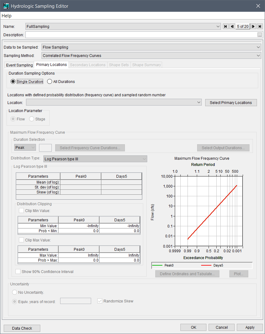
Primary Locations
The Primary Locations tab allows the user to select the primary inflow locations and define an annual Maximum Flow Frequency Curve, with Durations and Uncertainty, for each selected location. The list of available primary locations are derived from the common computation points (CCPs) defined in the watershed (for further details on CCPS, refer to the HEC-WAT User's Manual). The hydrologic sampling algorithm for this method uses correlated random sampling to generate a random flow magnitude from an uncertainty-adjusted probability distribution (maximum flow frequency curve) for each defined primary location for each event. A Primary location may sample either flow or channel stage. Additionally, if there is more than one relevant duration, frequency curves may be specified for several durations, with various available options for choosing one or all durations for scaling hydrographs.

The structure of the Primary Locations tab consists of three panels that change with Location, which are Duration(s), Maximum Flow Frequency Curve, and Uncertainty. As described in the following subsection, users create a list of primary locations and then enter information specific to each primary location.
Important
Each primary location has a separately defined Location Parameter, Duration(s), Maximum Flow Frequency Curve, and Uncertainty that the user must specify. Modifying the default Duration Output is optional. Data Check (Section 1.2.6) notifies the user if primary locations are incomplete (missing any required user inputs). When input data for a primary location has not been completed, and data check has been run (clicked Data Check), a Message window will display listing issues for a primary location.
Duration Sampling Options
The first step to completing the Primary Locations tab is to set the duration sampling option, from the Duration Sampling Options panel select either Single Duration or All Durations.
Creating Primary Locations
Select Primary Locations
The second step is to select the primary inflow locations:
- From the Primary Locations tab, click Select Primary Locations, the Selection Editor will open. From the Selection Editor, users will identify primary locations from the list of common computation points defined for the study watershed (e.g., Bluestone Inflow Near Glen Lynn).

From the Selection Editor, select the required primary locations from the Available Locations list (e.g., Tornado), click Add. This will move the selected locations to the Selected Locations list. The Add All button moves all Available Locations to the Selected Locations list. Alternatively, double-clicking on a location in the Available Locations list will move the selected location to the Selected Locations list.

Note
For users editing an existing hydrologic sampling alternative when secondary locations have previously been selected (review Secondary Locations), secondary locations previously added are displayed with "~Sec:" in front of the location name (e.g., ~Sec: Charleston Lock 6) at the bottom of the Available Locations list, as displayed in the Section Editor. The "~Sec:" indicates that those locations were already selected as secondary locations, and should therefore not be selected as primary locations.
To remove locations from the Selected Locations list, either click Remove for individually selected locations, or click Remove All to remove all selected locations.
Note
Users can add or remove selected locations at any time. However, if users attempt to remove primary locations, a Location Selection Warning message opens, and requires users to confirm the deletion of the primary location and all related information.

- Following the successful selection of the primary location(s), click OK, the Selection Editor will close.
- A list of the primary locations will be available from the Location list.
- For each primary location, the user must specify the location-specific Flow or Stage choice, Duration, Maximum Flow Frequency Curve, and the Uncertainty for each primary location.
Select Location Parameter
For each primary location selected (review Select Primary Locations), set the Location Parameter as either Flow or Stage. When Stage is selected the user must enter a Reference Stage

Define Maximum Frequency Curve(s)
Next, users need to enter information for the maximum flow or stage frequency curve. This information includes selecting a duration, and selecting the distribution type (Log Pearson Type III, Log Normal, GEV, Empirical) and defining the corresponding inputs for the selected distribution type.
Duration Selection
A maximum flow frequency curve is the probability distribution of annual maximum or coincident flows that represents either an instantaneous peak or an average flow across some duration. From the Duration Selection panel of the Hydrologic Sampling Editor; in the Maximum Flow Frequency Curve panel, the user can select either an instantaneous peak, number of days, or number hours of duration for the selected primary location. If more than one duration is needed for scaling events, additional durations may be specified, with a frequency curve for each. Multiple durations are specified with the "select frequency curve durations button.
Add Duration(s)
Users can add additional durations and exceedance probability ranges by clicking Select Frequency Curve Durations, from the Duration Selection panel. The Add Duration dialog box opens.

Click the Add Duration button to open the Add Duration dialog. Select the Granularity (e.g., Hours) and enter the Number (e.g., 48), click OK to add to the entered duration to the table (e.g., Hours48) and set the exceedance probability maximum (e.g., 0.1).

The table automatically orders created durations with the longest duration in the bottom row (e.g., Hours72). To remove a duration, select the desired row and click Remove Duration. The plot window displays a summary of the exceedance probabilities to sample a given duration. When complete, click OK to save the entered durations and exceedance probability ranges. The user is now retuned to the Hydrologic Sampling Editor and the selected durations are added as columns to the frequency curve distribution input table in the Distribution Type panel.
Duration Output
One or more primary locations must be defined (review Creating Primary Locations) before a user can specify duration outputs.
The hydrologic sampling algorithm automatically stores outputs for the duration(s) defined by the user from the Duration Selection panel including if additional frequency curve durations are selected (from the Add Durations dialog box). The Duration panel also contains an optional item, the Select Output Durations button which opens the Duration Output dialog. The Duration Output dialog allows users to store average event flows of additional durations, or an instantaneous peak, as output. The hydrologic sampling output variables and DSS output include the flow magnitude for the duration specified for the frequency curve as MAX FLOW, and all other durations as specified.

Note
Users must access the HEC-WAT Output Variable Editor to select the desired duration outputs to save the provided hydrologic sampling DSS output (e.g., MAX FLOW, PEAK FLOW, AVG 3 DAY MAX). Review the HEC-WAT User Manual available here: HEC-WAT Documentation for more information on the Output Variable Editor, accessing output variable results and accessing DSS (*.dss) result file(s).
To set the output durations:
- From the Duration Output dialog box, from the Duration Units, select one of the available options (Days or Hours) from the list in the cell. The selection (e.g., Hours) will activate the corresponding Duration Value cell.
- Next, in the activated Duration Value cell, enter the desired value (e.g., 72.0, which adds a duration output for the maximum 72-hour average flow).
- Duration units include:
- Inst. Peak (Instantaneous Peak) – this option is the default and cannot be modified or removed.
- Days – once selected to the right, in the box, enter the number of days for the duration value.
- Hours – once selected to the right, in the box, enter the number of hours for the duration value.
- Enter the desired number of additional durations to include in the hydrologic sampling output. Entered duration units and duration values can be modified at any time.
- To edit the Duration Output table, right-click on cells in the table on the Duration Output dialog box. Each column has its own unique shortcut menu (table shortcut options are described in Hydrologic Sampling Editor Interface, Tables section) with various options for editing the Duration Output table.
- Click OK, the Duration Output dialog box will close, and the edits will be saved. The user is now retuned to the Hydrologic Sampling Editor.
Select and Define the Distribution Type
From the Maximum Flow Frequency Curve panel, from the Distribution Type list select the desired distribution type.
Note
A column is added to the distribution table for each of the durations selected (as described in the Duration Selection section). Users must enter the parameters for both durations in the distribution table.

Distribution type options include: Normal, Log Normal (base 10), Pearson type III, Log Pearson type III (default curve), Generalized Extreme Value (GEV) and Empirical (graphical). Here is an overview of each of the distributions types:
- The default distribution type is Log Pearson type III. To define a Log Pearson Type II distribution the user must enter the Mean (of log), St. dev (of log) (standard deviation), and the Skew (of log) distribution parameters. Note, the user has the option to clip the lower or upper tail of the distribution using the Clip Min Value, or Clip Max Value, or both (see the section on Clipping the Lower and/or Upper Tails of a Frequency Curve).

- If the Pearson Type II distribution is selected, the user must enter the Mean, St. dev (standard deviation), and the Skew distribution parameters. Note, the user has the option to clip the lower or upper tail of the distribution using the Clip Min Value, or Clip Max Value, or both (see the section on Clipping the Lower and/or Upper Tails of a Frequency Curve).
- For a Normal distribution, the user will the following parameters: Mean and St. dev (standard deviation). Users can has the option to clip the lower or upper tail of the distribution using the Clip Min Value, or Clip Max Value, or both (see the section on Clipping the Lower and/or Upper Tails of a Frequency Curve).
- For the Log Normal (base 10) distribution, the user will the following parameters: Mean (of log) and St. dev (of log) (standard deviation). Users can has the option to clip the lower or upper tail of the distribution using the Clip Min Value, or Clip Max Value, or both (see the section on Clipping the Lower and/or Upper Tails of a Frequency Curve).
- The Generalized Extreme Value (GEV) distribution require that the following distribution parameters be entered, Location (ξ), Scale (α), and Shape (κ). The Maximum Flow Frequency Curve Plot automatically updates when user inputs are changed. Note, the user has the option to clip the lower or upper tail of the distribution using the Clip Min Value, or Clip Max Value, or both (see the section on Clipping the Lower and/or Upper Tails of a Frequency Curve).
Note
The GEV input parameters can be defined in more than one way. In the Hydrologic Sampler (HEC-WAT Version 1.0 and greater) and HEC-SSP (Version 2.2 or greater) software packages, the GEV input parameters follow the description in the Handbook of Hydrology (Maidment Ed., 1993) and Regional Frequency Analysis (Hosking et. al., 1997).
- The Empirical (graphical) distribution requires that a user complete the Exceedance Probability and Flow (cfs) table. By right-clicking on a cell in the table, a shortcut menu will display with options (e.g., cut, copy, paste, etc.) for editing the table (refer to the Hydrologic Sampling Editor Interface, Tables section). Note, extrapolation does not occur beyond the user-defined minimum and maximum flow. The Maximum Flow Frequency Curve Plot automatically updates when user inputs are changed.
 distribution.")
When defining the maximum flow (or stage) frequency curve, users must select a distribution type and define the corresponding distribution parameters. For the distribution types (other than Empirical), the user may choose to "clip", or constrain, the entered distribution to a defined minimum or maximum value, to limit the range of values sampled. The probability across the unconstrained range of the distribution is then increased by the excluded probability. Clipping limits are defined by selecting Clip Min Value and/or Clip Max Value, and entering a value for either the minimum or maximum value (see the section on Clipping the Lower and/or Upper Tails of a Frequency Curve). HEC-WAT automatically creates the probability, which automatically updates the maximum flow frequency curve. The Empirical distribution requires users to enter a table of exceedance probability versus flow (cfs).
Viewing the Maximum Flow (or Stage) Frequency Curve
Whatever method the user chooses to generate a maximum flow frequency curve, a plot of the curve is displayed on the Hydrologic Sampling Editor. This plot automatically updates when user inputs are changed. In addition, by clicking Plot, the Maximum Flow Frequency Curve dialog box will open displaying a plot of the current maximum flow frequency curve. This allows the user to examine the resultant plot of the defined curve in more detail. Refer to Hydrologic Sampling Editor Interface for more details regarding plots in the Hydrologic Sampling Editor.

In addition, users can view a tabulated report that displays the calculated flow values and default exceedance probability ordinates of the maximum flow frequency curve. To view the table, click Define Ordinates and Tabulate, the Define Ordinates and Tabulate Distribution dialog box will open (as described in the Default Exceedance Probability Ordinates section).
Default Exceedance Probability Ordinates
The Define Ordinates and Tabulate Distribution dialog box displays the probability versus flow table for the defined probability distribution. The displayed values represent both the original distribution and the result of imposed boundaries; i.e., the optional minimum or maximum clipping thresholds. The hydrologic sampling algorithm calculates flow (cfs) values based on the entered input parameters for the selected distribution and the default list of exceedance probability ordinates.

The user can modify/add/remove exceedance probability ordinates and the changes do not affect the entered distribution in any way. However, changes are reflected in the computed quantiles and the plot of the maximum flow frequency curve. Specifically, if the user adds or removes exceedance probability ordinates, the plot of the maximum flow frequency curve will update and display the values contained in the table at any given time. To modify, remove or add additional exceedance probability ordinates to the maximum flow frequency curve:
- From Maximum Flow Frequency Curve panel; click Define Ordinates and Tabulate, the Define Ordinates and Tabulate Distribution dialog box will open.
- It is not necessary to overwrite or add new exceedance probability ordinates in numerical order. When done with modifications, close the Define Ordinates and Tabulate Distribution dialog box. Upon reopening the dialog box, new/modified exceedance probabilities are automatically reordered, with corresponding flows generated.
- To overwrite an existing Exceedance Probability, click inside the cell and enter the desired probability.
- To remove existing exceedance probability ordinates, select the cell (or multiple cells) that contains the exceedance probability ordinate(s) to be deleted. Right-click on that cell, from the shortcut menu (review Hydrologic Sampling Editor Interface for more information regarding tables), click Delete Row(s). The selected exceedance probability ordinate(s) are removed from the table.
- To enter additional exceedance probability ordinates, right-click on a selected cell, from the shortcut menu, click Insert Row(s). The Insert Rows dialog box will open, in the Number to insert box, enter the number of new rows needed. Click OK, the Insert Rows dialog box will close, and blank cell(s) will display above the cell that was selected. Enter an exceedance probability ordinate(s) in the new cell(s), once the user leaves that cell(s), the associated flow value will automatically update based on the entered exceedance probability ordinates(s).
- Manual edits to the values in the Flow (cfs) column are not allowed as the flows are calculated based on the exceedance probability distribution. However, the user can manipulate the Flow (cfs) column, by right-clicking on the column, and accessing commands from the shortcut menu.
- Once editing is complete, click OK, the Define Ordinates and Tabulate Distribution dialog box will close. Modifications made to the exceedance probability ordinates(s) will automatically be saved, and the Maximum Flow Frequency Curve plot will atomically update.
Clipping the Lower and/or Upper Tails of a Frequency Curve
For the Log Pearson type III, Log Normal, and GEV distribution types, the user can clip the lower or upper tail of a distribution using the Clip Min Value, or Clip Max Value, or both. This clipping or constraining of the entered distribution, defines the minimum or maximum value, which limits the range of values sampled. The probability across the unconstrained range of the distribution is then increased by the excluded probability.
For example, to clip the upper tail of a Log Pearson Type III distribution, select Clip Max Value, enter the maximum flow (cfs) value (e.g., 11000). The Prob > Max box will automatically update (e.g., 0.0026 or 0.26 percent) to show the probability (a value between 0.0 – 1.0, not a percent) of the original distribution having a value beyond the clip threshold (and thus being clipped or excluded). The probability distribution is then adjusted so that the remaining range spans the excluded probability.

Uncertainty
The annual maximum flow frequency curve specified for each primary location is not known precisely, because the estimated curve is uncertain due to the limited available record length used to estimate it. This "sampling error" is an example of "knowledge uncertainty", as described in Introduction, and is randomized at the realization level (outer loop) of the HEC-WAT FRA nested Monte Carlo simulation, meaning it is sampled once per realization.
The uncertainty in the generated maximum flow frequency curve is incorporated by parametrically bootstrapping each frequency curve once per realization. In other words, a new frequency curve is generated by randomly sampling N values (where N is the equivalent record length) from the original frequency curve, and then re-estimating the parameters of the specified probability distribution from that N-value sample. Individual flow magnitudes are then sampled for each event (via HEC-WAT's inner loop sampling) from the uncertainty-adjusted frequency curves for the current realization (via HEC-WAT's outer loop sampling). For further details regarding the HEC-WAT Monte Carlo simulation, review the HEC-WAT User Manual available here: HEC-WAT Documentation.
From the Uncertainty panel, users need to enter information about the uncertainty of the maximum flow frequency curve. Generally, two uncertainty options are available for all distribution types: No Uncertainty, or a specified Equivalent Years of Record (default). A third option of User Defined Uncertainty is available for an Empirical (graphical) frequency curve, which uses a normal distribution at each ordinate with a user-defined standard deviation, entered as a table.

No Uncertainty
From the Uncertainty panel, select No Uncertainty. This option does not add uncertainty and the defined maximum flow frequency curve is used for sampling events in every realization.
Equivalent Years of Record
From the Uncertainty panel, select Equiv. years of record (default) and enter the number of years in the box next to Equiv. years of record. An equivalent record length parameterizes uncertainty due to a limited record length. This value is either the actual record length used to estimate the flow frequency curve, or an equivalent length based on either (a) the addition of historical information, (b) use of a regional skew, or (c) development of the frequency curve from a method other than a statistical analysis of a gaged or modified flow record.
For analytical distributions (Log Pearson type III, Log Normal, GEV, Empirical), the Equiv. years of record defines N (where N equals specified equivalent record length) to create the random "bootstrap" sample to generate the realization-specific frequency curve used for sampling events.
Randomize Skew – this option is only enabled when the selected distribution type is Log Pearson type III, and is enabled by default to be consistent with the uncertainty description in Bulletin 17C. When Randomize Skew is enabled (select the checkbox), the computation will use the skew coefficient computed from the bootstrap sample. Bulletin 17B uncertainty does not recognize the uncertainty in the skew coefficient, and if the user prefers to maintain consistency with Bulletin 17B, the user should not select the Randomize Skew option. In this case, the skew is not re-computed from the bootstrap sample, and instead the original user-entered skew coefficient is used.
User Defined Uncertainty
This option is only available when the selected distribution type is Empirical (graphical). Select User Defined Uncertainty to enable the table which displays default values. Edit the default values in the table to override the computed standard deviation of uncertainty for each frequency quantile, which is based on the order statistics method. Right-click inside the table to access the same shortcut menu options (e.g., cut, copy, paste, etc.) discussed the Hydrologic Sampling Editor Interface, Tables section.

Click Apply to save changes made to the Primary Locations tab. Alternatively, if a user is finished adding information or editing, click the OK to close the Hydrologic Sampling Editor. Users can click Data Check (review Hydrologic Sampling Editor Interface, Data Check section) to determine if any primary locations were missed before proceeding to the Secondary Locations tab (review Secondary Locations), if desired. Note, the Data Check is generally used after all required inputs have been defined to avoid generating a long list of as-yet undefined inputs (e.g., undefined Correlation Matrix and Shape Sets data).