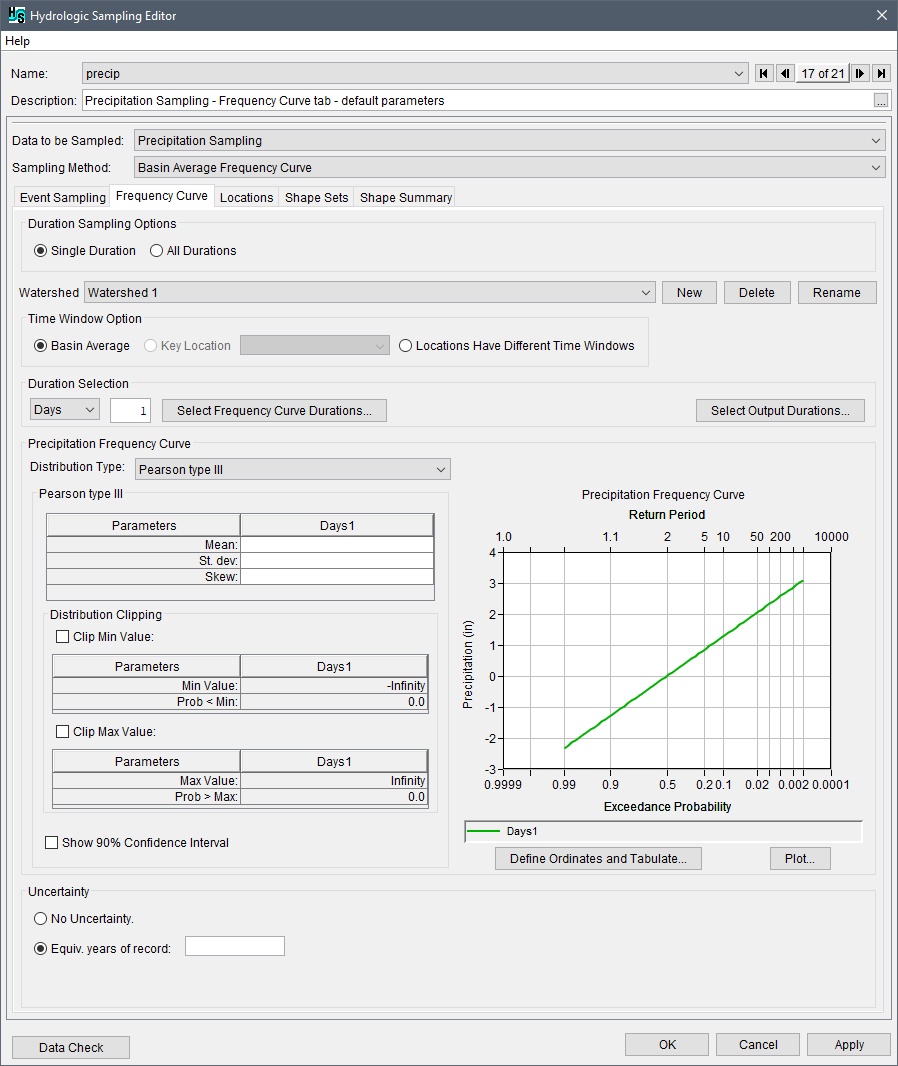
From the Hydrologic Sampling Editor, the Frequency Curve tab is where the annual maximum basin-average Precipitation Frequency Curve is defined for each watershed. The Frequency Curve tab allows users to set multiple-duration sampling options, define multiple watersheds, and to select the duration(s) and probability Distribution Type of precipitation frequency curve(s) and define its corresponding user inputs for each watershed. This tab also includes the ability for users to specify the Uncertainty for the defined precipitation frequency curve(s). 

As described in the introduction to this chapter, the Hydrologic Sampler generates a basin-average precipitation depth for every event by randomly sampling an event depth from the precipitation frequency curve. (With multiple watersheds defined, a correlated depth is sampled for each from its frequency curve.) A unique frequency curve is generated for each realization, fit to a parametric bootstrap sample of N equals EYR values, to capture the knowledge uncertainty about the user-entered curve. The sampled basin-average precipitation value is then "disaggregated" to each subbasin hyetograph location by scaling a randomly chosen shape set based on its initial subbasin area-weighted-average depth, in a process that maintains the area-weighted average. This process will reproduce the temporal and spatial distribution of rainfall in the watershed as represented by the user-defined shape set, with a range of event depths from the user-defined basin average precipitation frequency curve.

Precipitation Frequency Curve

Users should work through the Frequency Curve tab to define the precipitation frequency curve(s) from the top. For example the Watershed dropdown menu allows users to define the Time Window Option, Duration(s), Precipitation Frequency Curve and Uncertainty by watershed (the default watershed is Watershed 1).

Duration and Watershed Setup 

The first step to completing the Frequency Curve tab is to set the duration sampling option, from the Duration Sampling Options panel select either Single Duration or All Durations.  

The second step is to identify the watershed name(s) for the alternative. The default watershed is Watershed 1. Click New, to add a new watershed from the Create New Watershed dialog box. Users can also delete created watersheds by clicking the Delete button to open the Delete Watershed message dialog. Created watershed can be renamed by clicking the Rename button to open the Rename Watershed dialog box. 

Time Window Option

Next, for the selected watershed, from the Time Window Option panel, select the appropriate time window option from: Basin Average (default selection), Key Location (and location selection), or Locations Have Different Time Windows. 

Note

The option to set the time window to Key Location is disabled (cannot be completed) until at least one hyetograph location has been defined in the Locations tab (review Hyetograph Locations for more information). 

Duration Selection 

From the Duration Selection panel define the duration(s) for the precipitation frequency curve. By default, the duration is set to Days, 1. Use the dropdown menu to sent a different duration, options include Peak, Minutes, Hours, or Days (default). Enter a duration value in the box (default is set to 1).

Add Duration(s)

Users can add additional durations and exceedance probability ranges by clicking Select Frequency Curve Durations, from the Duration Selection panel.  The Add Duration dialog box opens.

Click the Add Duration button to open the Add Duration dialog. Select the Granularity (e.g., Hours) and enter the Number (e.g., 48), click OK to add to the entered duration to the table (e.g., Hours48) and set the exceedance probability maximum (e.g., 0.1). 

The table automatically orders created durations with the longest duration in the bottom row (e.g., Hours72). To remove a duration, select the desired row and click Remove Duration. The plot window displays a summary of the exceedance probabilities to sample a given duration. When complete, click OK to save the entered durations and exceedance probability ranges. The user is now retuned to the Hydrologic Sampling Editor and the selected durations are added as columns to the frequency curve distribution input table in the Distribution Type panel.

Duration Output

The hydrologic sampling algorithm automatically stores outputs for the duration(s) defined by the user from the Duration Selection panel including if additional frequency curve durations are selected (from the Add Durations dialog box). The Duration panel also contains an optional item, the Select Output Durations button which opens the Duration Output dialog. The Duration Output dialog allows users to store average event flows of additional durations, or an instantaneous peak, as output. The hydrologic sampling output variables and DSS output include the flow magnitude for the duration specified for the frequency curve as MAX FLOW, and all other durations as specified.

Note

Users must access the HEC-WAT Output Variable Editor to select the desired duration outputs to save the provided hydrologic sampling DSS output (e.g., MAX FLOW, PEAK FLOW, AVG 3 DAY MAX). Review the HEC-WAT User Manual available here: HEC-WAT Documentation for more information on the Output Variable Editor, accessing output variable results and accessing DSS (*.dss) result file(s).

To set the output durations:

1. From the Duration Output dialog box, from the Duration Units, select one of the available options (Days or Hours) from the list in the cell. The selection (e.g., Hours) will activate the corresponding Duration Value cell. 
2. Next, in the activated Duration Value cell, enter the desired value (e.g., 72.0, which adds a duration output for the maximum 72-hour average flow).
3. Duration units include:
   • Inst. Peak (Instantaneous Peak) – this option is the default and cannot be modified or removed.
   • Days – once selected to the right, in the box, enter the number of days for the duration value.
   • Hours – once selected to the right, in the box, enter the number of hours for the duration value.
4. Enter the desired number of additional durations to include in the hydrologic sampling output. Entered duration units and duration values can be modified at any time.
5. To edit the Duration Output table, right-click on cells in the table on the Duration Output dialog box. Each column has its own unique shortcut menu (table shortcut options are described in Hydrologic Sampling Editor Interface, Tables section) with various options for editing the Duration Output table.
6. Click OK, the Duration Output dialog box will close, and the edits will be saved. The user is now retuned to the Hydrologic Sampling Editor.

Precipitation Frequency Curve Distribution

After setting the duration(s), select the distribution type of the precipitation frequency curve from the Precipitation Frequency Curve panel. The distribution type has four options available: Pearson Type III (selected by default), Normal, GEV (Generalized Extreme Value), Kappa and Empirical (graphical). When completing the Precipitation Frequency Curve panel, users must select a distribution type and define its corresponding user inputs. Note, for the empirical distribution, a table of exceedance probability versus precipitation (total in inches) must be entered. To the right of the inputs or the input table is the Precipitation Frequency Curve plot, which displays the selected distribution based on the entered user inputs.

The Hydrologic Sampler automatically updates the plot for precipitation (in) calculated based on the user inputs for the entered distribution for a default list of exceedance probability ordinates. Users can open the Precipitation Frequency Curve plot for closer examination by clicking the Plot button, or by double-clicking inside the plot to open the graph in another window. Refer to Hydrologic Sampling Editor Interface, Plots for more details regarding plots in the Hydrologic Sampling Editor. Additional frequency ordinates can be computed and added to the plot. Those ordinates, and a tabulation of the precipitation depth at each ordinate, are displayed in a table opened by the Define Ordinates and Tabulate button. Users can insert and delete rows to change which ordinates are plotted.

For distributions other than Empirical (graphical), the user may choose to "clip," or exclude, the entered distribution beyond a defined minimum or maximum value, to limit the range of values sampled. Clipping limits are defined using the optional Clip Min Value and Clip Max Value checkboxes located below the user inputs. User-defined clipping thresholds automatically update the Precipitation Frequency Curve plot, as well as the table opened by the Define Ordinates and Tabulate button.

Viewing a Precipitation Frequency Curve

Whatever duration and distribution the user chooses to define a precipitation frequency curve, a plot of the curve is displayed on the Hydrologic Sampling Editor. This plot automatically updates when user inputs are changed. In addition, by clicking Plot, the Precipitation Frequency Curve dialog box will open displaying a plot of the current precipitation frequency curve. The plot allows the user to examine the resultant graph of the defined curve in more detail. Refer to Hydrologic Sampling Editor Interface for more details regarding plots in the Hydrologic Sampling Editor.

In addition, users can view a tabulated report that displays the calculated precipitation values for default exceedance probability ordinates of the precipitation frequency curve. To view the table, click Define Ordinates and Tabulate, the Define Ordinates and Tabulate Distribution dialog box will open. Furthermore, the table displayed in this dialog allows the user to extend the distribution graph to more extreme ordinates.

Default Exceedance Probability Ordinates

The Define Ordinates and Tabulate Distribution dialog displays the probability versus precipitation table for the defined probability distribution. The displayed values represent both the original distribution and the result of imposed boundaries; i.e., the optional minimum or maximum clipping thresholds. The Hydrologic Sampler calculates the Precipitation (in) based on the entered distribution inputs and the default standard list of Exceedance Probability ordinates.

Changes made in this dialog do not affect the distribution entered in the Precipitation Frequency Curve panel in any way. However, changes are reflected in the Precipitation Frequency Curve graph and quantiles displayed.

If the user adds or removes ordinates from the table, they can display more or less of the frequency curve in the plot window. From the Define Ordinates and Tabulate Distribution dialog, users can view, modify, remove or add additional ordinates to the Exceedance Probability column regardless of the distribution type selected. To open and view, modify, remove or add ordinates:

1. From the Precipitation Frequency Curve panel; click Define Ordinates and Tabulate, the Define Ordinates and Tabulate Distribution dialog box will open.
2. Note, when editing the exceedance probability ordinates, it is not necessary to overwrite or add new exceedance probability ordinates in numerical order. When done with modifications to the exceedance probability ordinated, close the Define Ordinates and Tabulate Distribution dialog. When opening the dialog box, new/modified exceedance probabilities are automatically reordered, with corresponding precipitation generated.
3. To overwrite an existing Exceedance Probability ordinate, click inside the cell and enter the desired probability.
4. To remove existing exceedance probability ordinates, select the cell (or multiple cells) that contains the exceedance probability ordinate(s) to be deleted. Right-click on that cell, from the shortcut menu, click Delete Row(s). The selected exceedance probability ordinate(s) are removed from the table.
5. To enter additional exceedance probability ordinates select a cell where the new exceedance probability ordinate(s) is to be added. Right-click on that cell, from the shortcut menu, click Insert Row(s). The Insert Rows dialog box will open, in the Number to insert box, enter the number of new rows needed. Click OK, the Insert Rows dialog box will close, and blank cell(s) will display above the cell that was selected. Enter exceedance probabilities in the new cell(s) and the Precipitation (in) column updates automatically.
6. Manual edits to the precipitation values are not allowed, as the precipitation values are calculated based on the exceedance probability distribution. However, the user can copy, print, or sum the Precipitation (in) column, by right-clicking on the column, and using the available shortcut menu commands.
7. Once editing is complete, click OK, and the Define Ordinates and Tabulate Distribution dialog box will close. Modifications made to the exceedance probability ordinates(s), with resulting precipitation depth(s), will automatically save and update the Precipitation Frequency Curve plot.

Select and Define the Distribution Type

From the Precipitation Frequency Curve panel, from the Distribution Type list select the desired distribution type.  

Note

A column is added to the distribution table for each of the durations selected (as described in the Duration Selection section). Users must enter the parameters for both durations in the distribution table.

Distribution type options include: Pearson type III (default curve), Normal, Generalized Extreme Value (GEV), Kappa and Empirical (graphical). Here is an overview of each of the distributions types:

• The default distribution type is Pearson type III. To define the Pearson type III distribution the user must enter the Mean, St. dev (standard deviation), and the Skew distribution parameters. Changes made to the parameters immediately update the Precipitation Frequency Curve graph. The following figure provides an example of a completed Pearson Type III distribution and the resulting frequency curve graph. Note, the user can opt to clip the lower or upper tail of the distribution using the Clip Min Value, or Clip Max Value, or both (see the section on Clipping the Lower and/or Upper Tails of a Frequency Curve).
• To define the Normal, enter the Mean and St. Dev (standard deviation) distribution parameters. Changes made to the parameters immediately update the Precipitation Frequency Curve graph. Note, the user can opt to clip the lower or upper tail of the distribution using the Clip Min Value, or Clip Max Value, or both (see the section on Clipping the Lower and/or Upper Tails of a Frequency Curve).
• To define the GEV (Generalized Extreme Value), enter the Location (ξ), Scale (α) and Shape (κ) distribution parameters. Changes made to the parameters immediately update the Precipitation Frequency Curve graph. Note, the user can opt to clip the lower or upper tail of the distribution using the Clip Min Value, or Clip Max Value, or both (see the section on Clipping the Lower and/or Upper Tails of a Frequency Curve).

Note

The GEV user parameters can be defined in more than one way. In HEC-WAT (Version 1.0) and HEC-SSP (Version 2.2 or greater) software, the GEV input parameters follow the description in the Handbook of Hydrology (Maidment Ed., 1993) and Regional Frequency Analysis (Hosking et. al., 1997).

• To define the Empirical (graphical) distribution type, complete the Exceedance Probability and Precipitation (in) table using manual entry, or copy in from another table. Precipitation (in) refers to precipitation total in inches. Right-click inside the table to access the shortcut menu options available (e.g., cut, copy, paste, etc.) for editing the table (refer to Hydrologic Sampling Editor Interface for shortcut options). Note, extrapolation does not occur beyond the user-defined minimum and maximum precipitation, so the curve must be defined for the desired sampling range. Changes made to the inputs immediately update the Precipitation Frequency Curve graph.

• A Kappa distribution requires the user to enter a Location, Scale, Shape 1, and Shape 2 distribution parameters. Note, the user can opt to clip the lower or upper tail of the distribution using the Clip Min Value, or Clip Max Value, or both (see the section on Clipping the Lower and/or Upper Tails of a Frequency Curve).

Clipping the Lower and/or Upper Tails of the Frequency Curve

For Pearson type III, Normal, and GEV distribution types, the user can opt to clip the lower or upper tail of a distribution using Clip Min Value (Prob < Min), or Clip Max Value (Prob > Max). For example, it is good practice to clip the lower tail at 0.0 to prevent negative values. 

To create clipping threshold(s), check the checkbox next to the clipping option (Clip Min Value and/or Clip Max Value) to select it. Once selected, the value field is enabled. Enter the minimum or maximum value in the enabled field, and the corresponding Prob < Min or Prob > Max field updates showing the probability of the original distribution having a value beyond the clip threshold (and thus being clipped, or excluded from the precipitation frequency curve).

Note

The calculated probability is displayed as a value between 0.0 – 1.0, not a percent. The example clipped GEV distribution used the Clip Min Value option. In this example, the Clip Min Value of 0 inches results in a probability (Prob > Min) of 0.0210 (or 2.1 %). It is strongly recommended that a minimum clip value of 0.0 be defined for precipitation sampling, even if the frequency curve does not closely approach zero. This choice ensures that each re-sampled realization-specific frequency curve, which may be lower than the original user-entered curve, is also kept greater than zero.

Uncertainty

The Hydrologic Sampler includes the ability to capture uncertainty when the specified basin average precipitation frequency curve is not known precisely (e.g., due to limited available record length). This type of uncertainty is knowledge uncertainty (as described in the Introduction), and is addressed in the outer loop of HEC-WAT Flood Risk Analysis (FRA) nested Monte Carlo simulation, meaning it is sampled once per realization.

As noted in the introduction to this chapter, a new frequency curve is generated for each realization by parametrically bootstrapping, or randomly sampling N values (where N is the equivalent record length) from the original frequency curve, and then fitting a new frequency curve of the same distribution type with parameters estimated from that N-value sample. This new frequency curve is generated in the outer loop of the HEC-WAT Monte Carlo simulation. All event precipitation magnitudes are then sampled from this uncertainty-adjusted frequency curve, in the inner loop of the HEC-WAT Monte Carlo simulation (review the Introduction).

From the Hydrologic Sampling Editor, enter information about the uncertainty of the precipitation frequency curve from the Uncertainty panel of the Frequency Curve tab. Generally, two uncertainty options are available for all distribution types that users may choose from: No Uncertainty, or a specified Equivalent Years of Record (default). A third option is available to define uncertainty for an Empirical (graphical) frequency curve (User Defined Uncertainty), which uses a normal distribution at each ordinate with a user-defined standard deviation, entered as a table.

No Uncertainty

From the Frequency Curve tab; from the Uncertainty panel, select No Uncertainty. Choose this option to use the user-defined precipitation frequency curve for sampling events in every realization without adding uncertainty.

Equivalent Years of Record

From the Uncertainty panel, select Equiv. years of record (default) and enter the number of years in the box next to Equiv. years of record. An equivalent record length parameterizes uncertainty due to a limited record length. This uncertainty value is either the actual record length used to estimate the precipitation frequency curve, or an equivalent length based on the regional analysis used to develop the precipitation frequency curve.

For analytical distributions (Uniform, Triangular, Normal or Gamma), a new frequency curve is generated by creating a random "bootstrap" sample of size N (where N = specified equivalent record length) from the originally entered frequency curve, and re-estimating the distribution parameters from that sample.

User Defined Uncertainty

This option is only available when the selected Distribution Type is Empirical (graphical). From the Uncertainty panel, select the User Defined Uncertainty option, this enables the provided table, which displays default values of standard deviation. If necessary, edit the default values to override the computed standard deviation of uncertainty for each frequency quantile (based on the order statistics method). Right-click inside the table to access the same shortcut menu options (e.g., cut, copy, paste, etc.) discussed Hydrologic Sampling Editor Interface.

Click the Apply button to save changes made to the Frequency Curve tab. Alternatively, if users are finished adding information or editing, then click the OK button to close the Hydrologic Sampling Editor. Users can click the Data Check button (review Hydrologic Sampling Editor Interface) to determine if data consistency error(s) are present for the completed tab, before proceeding to the next tab, if desired. Note, the Data Check is generally used after all required inputs have been defined to avoid generating a long list of as-yet undefined inputs (e.g., undefined Hyetograph Locations and Shape Sets tabs).