Precipitation Sampling - Basin Average

This chapter describes how to set up the Hydrologic Sampler with a precipitation-sampling alternative using the Basin Average Frequency Curve sampling method. This sampling method generates a hyetograph for every specified subbasin location within the modeled watershed for each sampled event based on: a user-defined basin average precipitation depth-frequency curve, hyetograph shape sets and a flood season distribution. These hyetographs are then available for subsequent models in the HEC-WAT model sequence. The Basin Average Frequency Curve sampling method in the Hydrologic Sampler is described below and the user input steps are described in the following sections:

The Basin Average Frequency Curve sampling method is similar to the Correlated Flow Frequency Curves sampling method for sampling flow (refer to Chapter 2) in that event magnitudes are generated from user-defined frequency curves, and event time series are scaled to those magnitudes from user-provided shape sets. Specifically, an annual maximum basin-average frequency curve and its uncertainty must be specified by the user, and a basin-average precipitation depth is randomly sampled from it to generate the total storm depth for each event. However, a primary difference between the two methods is whether the frequency curves are aggregated or site-specific. Flow is sampled separately at various sites from site-specific flow frequency curves, while precipitation sampling uses an aggregated basin-average precipitation frequency curve. The randomly sampled precipitation depth is "disaggregated" (as described below) into precipitation hyetographs for user-specified subbasin locations. (The user may also define multiple watersheds, each having a basin-average precipitation frequency curve and subbasin locations, as described below.)

For A Single Watershed

Defining a single watershed is the most common use case, and will be described first. Discussion of multiple watersheds is below.

As noted above, a spatially aggregated basin-average precipitation frequency curve is randomly sampled to produce a storm depth for each event. The frequency curve describes the likelihood of precipitation depth over some duration of time. When the frequency curve is generated, the duration must be chosen carefully to capture a "critical" duration for the watershed, reflecting the duration of extreme precipitation events having the greatest effect on the resulting peak streamflow, and/or reservoir stage. If necessary, multiple durations may be specified, each with an associated frequency curve, that are sampled in concert. It is good practice for the duration of effective (non-zero) precipitation defined in the shape sets (described below) to match the duration of the frequency curve, or the longest duration if more than one duration and associated frequency curve is specified.

The user-defined uncertainty in the basin-average precipitation depth frequency curves is incorporated into the compute by parametrically bootstrapping each frequency curve once per realization. This process samples N basin-average depth magnitudes from the curve (where N is equal to the specified equivalent record length) and then re-fits a new frequency curve to that sample. All event depths for that realization are then sampled from the uncertainty-adjusted precipitation frequency curve, rather than the original user-specified frequency curve.

For each generated event, the set of precipitation time series generated by the Hydrologic Sampler (one for every subbasin location) is created by scaling a randomly chosen user-defined shape set. In this method, a shape set contains scalable hyetographs for every subbasin location that together capture the relative spatial and temporal distribution of rainfall throughout the watershed for a given event. A shape set is usually defined by a large event from the historical record, and is a unique instance of how precipitation occurred in both space and time. For example, one shape set might contain an event centered over the upper part of a watershed while another shape set is an event centered in the lower half of the watershed. When snowmelt is involved in HEC-WAT model sequence, temperature locations may also be specified and time-series provided in each shape set, although these time-series are not scaled but used exactly as defined.

The scaling of a user-defined shape set, such that the shape set's area-weighted average precipitation depth matches the randomly sampled value, is how the sampled basin-average precipitation depth is "disaggregated" to the subbasins. A weighted basin-average precipitation depth is computed for each shape set by summing the total precipitation depth within the maximum duration-window of the hyetograph for each subbasin, weighting it by the subbasin drainage area's percent of total area, then summing subbasin totals. Once an event depth is sampled from the basin-average precipitation frequency curve and a shape set is randomly chosen, that sampled depth is divided by the selected shape set's depth to compute a scaling ratio. This ratio is then used to scale the hyetograph of every subbasin to generate an event that reproduces the sampled basin average depth, i.e. all of the hyetographs are scaled by the same ratio, which adjusts their area-weighted basin-average depth to the sampled value.

Unlike flow sampling (refer to Correlated Flow Frequency Sampling), in which the entire shape set is scaled, the period of the hyetographs scaled is only the maximum duration window for the specified duration. When more than one duration is specified, the shortest window is scaled first, and then held while surrounding windows of longer durations scaled, making a nested, balanced event.

Finally, the scaled hyetographs are placed on a date that is randomly sampled from the flood season distribution defined by the user. The flood season is a probability distribution of event month and day, estimated from the dates of significant events in the watershed's observed record, sometimes including those that are not the annual maximum. In the absence of a gage record, familiarity with local hydrology can suggest a flood season probability distribution. Once the date for a flood event is randomly sampled, the peak of the final scaled hyetographs is placed on that date.

Defining Multiple Watersheds

While each basin-average frequency curve is aggregated for a watershed and its subbasins, the user may define multiple watersheds in a HS alternative, each having a frequency curve and subbasins. The frequency curves for the various watersheds are given specified spatial correlations and are jointly sampled for each event, similarly to the Correlated Flow Frequency Curves method described in Correlated Flow Frequency Sampling. (The simplest case is a single hydrologic sampler watershed and its subbasins, and it will by default receive the name "Watershed 1".)

When multiple watersheds have been defined, each shape set includes all the subbasin locations of all the watersheds included in the hydrologic sampling alternative. However, those locations are grouped and their hyetographs scaled by watershed. Specifically, for each shape set, a weighted basin-average depth is computed for each watershed from only its locations, and those location's hyetographs are scaled together such that the basin-average depth matches the depth sampled for that watershed from its precipitation frequency curve. Similar scaling is performed for each watershed to provide hyetographs for all locations for each event.

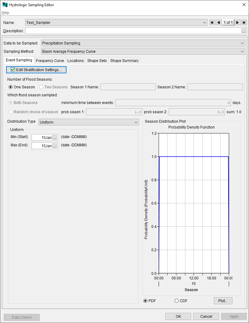
First, either create a new hydrologic sampling alternative (refer to Create a Hydrologic Sampling Alternative), or edit an existing alternative (review Individual Hydrologic Sampling Alternatives). From the Hydrologic Sampling Editor, from the Data to be Sampled list, select Precipitation Sampling. From the Sampling Method list, select Basin Average Frequency Curve.

Stratified Sampling

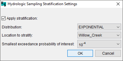
Stratified sampling in the Hydrologic Sampler changes the distribution of points along the frequency curve sampled. This sampling method can be used to increase emphasis in samples along a certain portion of the frequency curve, reducing the number of total events needed to represent the upper end of the curve.  By default stratified sampling is turned off and any point along the frequency curve is equally likely to be sampled (equivalent to a uniform distribution).  However, when stratified sampling is turned on the probabilities sampled along the frequency curve are weighted by a distribution identified by the user.

To enable stratified sampling and change the settings, click the Edit Stratification Settings button to open the Hydrologic Sampling Stratification Settings dialog. Check the Apply Stratification checkbox to turn on stratified sampling and select a distribution (Gumbel (EV1), Normal, Half-Normal, Exponential, and Uniform) and the location to apply stratified sampling to. The parameters for each distribution predefined and cannot be modified by the user. The Smallest exceedance probability of interest setting is used to set the probability at which the final stratification bin should begin.

Stratified sampling divides the frequency curve into bins based on the distribution selected and smallest exceedance probability of interest.  The number of bins are determined by the number of events within the lifecycle (number of years the analysis period spans). For example a 50-year analysis period will include 50 bins in the stratification. This process ensures that each lifecycle has a sample in every bin. Over the course of generating a set of sampled events in a lifecycle, each bin is sampled in order. The width of each bin is used in re-aggregation and summarization of model results. The probability of each bin is saved to a paired data record in the output variable DSS file for the compute.

Note

Stratified sampling cannot be used with multiple season sampling (e.g. when Two Seasons) is selected. Also, if the Edit Stratification Settings button does not display a checkmark then the Apply stratification checkbox in the Hydrologic Sampling Stratification Setting dialog box was not checked.

Single or Multiple Watersheds:

When the Basin Average Frequency Curve option is selected, the Hydrologic Sampling Editor interface will change based on the selected method. The Hydrologic Sampling Editor set to apply the Basin Average Frequency Curve sampling method contains the following five tabs: