Defining Precipitation Sampling Season
From the Hydrologic Sampling Editor, from the Event Sampling tab, the user can set the flood season. The flood season defines when precipitation events might occur within a year, and is described as a probability distribution of possible flood dates (day-month). Users can describe the probability distribution for the flood season using one of five distribution types (Uniform, Triangular, Normal, Gamma and Empirical).

The flood season can be as simple as a Uniform distribution between a minimum to maximum date, allowing the selection of any date in the range with equal likelihood. The flood season can also be a more complex distribution with some dates more likely than other dates. When an analytical distribution type is chosen (Uniform, Triangular, Normal or Gamma), the corresponding user inputs needed for that distribution must be entered.
The default values for minimum (start) and maximum (end) dates are 1 January (01Jan) and 31 December (31Dec), respectively, though the user may enter their own values to define the flood season bounds. For Normal and Gamma distributions, which do not have explicit upper and lower bounds, user-specified start and end dates may truncate the tails of the distribution.
Note
When the defined flood season distribution spans January 1, minimum and maximum dates must be re-defined from the defaults. Another distribution option is to create a user-defined non-parametric empirical (graphical) distribution, which requires a table of cumulative probability versus date entered by the user.
As explained in the introduction to this chapter, the sampled date is used to place the peak of the flood event hyetograph in time, as defined by the sampled and scaled shape set (refer to Hyetographs to Scale (Shape Sets)). Because different locations within a watershed might have different relative peak dates within a shape set's time-window, the location with the largest total hyetograph depth is used to match the peak to the sampled date.
Flood Season Definition
The Flood Season Definition panel of the Hydrologic Sampling Editor allows the user to select a probability distribution type from five options (Uniform (default), Triangular, Normal, Gamma and Empirical), specify the distribution's corresponding user inputs, as well as set the season start, and end dates. The Start and End dates are user inputs, which function differently for different distribution types. For the first two distributions, Uniform and Triangular, the start and end dates are explicit distribution inputs. However, for the second two distributions, Normal and Gamma, the start and end dates can be used to truncate the season distribution.
Default dates are 01Jan and 31Dec, and these must be re-defined if the flood season spans January 1 (e.g., when using a standard water year, from 1 October to 30 September). As the last step in the event generation algorithm, the hydrologic sampling algorithm randomly samples this user-defined flood season distribution to set the date (as day and month) of each flood event. The user must select the most representative distribution and define its corresponding user inputs accordingly.
Multiple Seasons
In some regions, flood events may be generated by different storm-producing mechanisms, often at different times of the year. An example is the Pacific Northwest, which has snowmelt runoff floods in the spring and rainfall-driven floods in the winter. These flood types have different durations with different magnitude-frequency relationships, and occur during different seasons. The Hydrologic Sampler therefore has the ability to specify two flood sampling seasons, each with a complete description of the probabilistic structure of floods, including season distribution, frequency curves, and event shapes.
By selecting Two Seasons under the Number of Flood Seasons setting, the user may define a second flood season to be sampled and all following settings must be defined for both seasons. The user may enter names for both seasons, and these names will be used in other tabs where information is required separately for each season. The only information common to both seasons is the hyetograph locations. The user may specify Both Seasons to be sampled in a single event or use Random choice of season to sample an event from either season based on a likelihood of each.
If Two Seasons are used, and sampling of Both Seasons is selected, the two seasons may overlap. The minimum time between events is used to ensure that the two sampled floods for a given event are adequately spaced.
Uniform Distribution
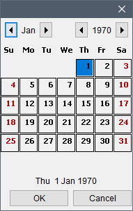
Uniform distribution is the default uncertainty distribution. Under the uniform distribution, the event is equally likely to occur on any day between two dates. The Uniform distribution includes two inputs - Min (Start) and Max (End). Defaults are 01Jan (Min) and 31Dec (Max). The user can edit these values manually (DDMMM), or by clicking ![]() . The Select Date dialog box will open that will allow the user to select a day and month. When the defined flood season distribution spans 1 January, minimum and maximum dates must be redefined. Changes made to the inputs immediately updates the Season Distribution Plot box of the Hydrologic Sampling Editor.
. The Select Date dialog box will open that will allow the user to select a day and month. When the defined flood season distribution spans 1 January, minimum and maximum dates must be redefined. Changes made to the inputs immediately updates the Season Distribution Plot box of the Hydrologic Sampling Editor.
, displaying the Probability Density Function plot with default values.")
Triangular Distribution
The Triangular distribution includes three inputs – Min (Start), Mode, and Max (End) dates. Defaults are 01Jan (Min), 01Jul (Mode), and 31Dec (Max). The user can edit these values manually (DDMMM), or by clicking the ![]() button. The Select Date dialog box will open that will allow the user to select a day and month. When the defined flood season distribution spans 1 January, minimum and maximum dates must be redefined from the defaults. Changes made to the inputs immediately updates the Season Distribution Plot box of the Hydrologic Sampling Editor.
button. The Select Date dialog box will open that will allow the user to select a day and month. When the defined flood season distribution spans 1 January, minimum and maximum dates must be redefined from the defaults. Changes made to the inputs immediately updates the Season Distribution Plot box of the Hydrologic Sampling Editor.

Normal Distribution
The Normal distribution includes four inputs – Mean, standard deviation (Std Dev.), Min (Start), and Max (End). Default values are 01 Jul (Mean), 20 (Std Dev.), 01Jan (Min), and 31Dec (Max). The user can edit the Mean, Min, and Max values manually (DDMMM); or by clicking ![]() . The Select Date dialog box will open that will allow the user to select a day and month. Std Dev. is entered in days. Changes made to the inputs immediately updates the Season Distribution Plot box of the Hydrologic Sampling Editor.
. The Select Date dialog box will open that will allow the user to select a day and month. Std Dev. is entered in days. Changes made to the inputs immediately updates the Season Distribution Plot box of the Hydrologic Sampling Editor.

The Normal distribution does not have explicit upper and lower bounds; therefore, the user-specified start and end dates can optionally be used to truncate the tails of the distribution resulting from the user-defined mean and standard deviation. However, the start and end dates must be redefined when the season spans 1 January; an example is provided for a season starting 1 November and ending 30 April.

Gamma Distribution
The Gamma distribution includes five inputs – Shape, Scale, Shift, Min (Start), and Max (End). Defaults are 2 (Shape), 20 (Scale), 0 (Shift), 01Jan (Min), and 31Dec (Max). The user can edit the Mean and Max values manually (DDMMM); or by clicking ![]() . A Select Date dialog box will open that will allow the user to select a day and month. Shape, Scale, and Shift are entered in days. Changes made to the inputs immediately updates the Season Distribution Plot box of the Hydrologic Sampling Editor.
. A Select Date dialog box will open that will allow the user to select a day and month. Shape, Scale, and Shift are entered in days. Changes made to the inputs immediately updates the Season Distribution Plot box of the Hydrologic Sampling Editor.

The Gamma distribution type does not have explicit upper and lower bounds; therefore, the user-specified start and end dates can optionally be used to truncate the season distribution resulting from the user inputs. However, the start and end dates must be redefined when the flood season spans 1 January.
Empirical (graphical) Distribution
For an Empirical, distribution a default Cumulative Probability function is provided. If necessary, the user can edit the Cumulative Probability Function, the Cumulative Probability column values must span from 0.0 to 1.0. The Date column values should be enter in the DDMM format, or by clicking ![]() . A Select Date dialog box will open that will allow the user to select a day and month. Changes made to the user inputs immediately update the Season Distribution Plot.
. A Select Date dialog box will open that will allow the user to select a day and month. Changes made to the user inputs immediately update the Season Distribution Plot.
 Distribution Type, displaying the Probability Density Function plot with default values.")
The Cumulative Probability function can be copied from an outside source (e.g., Microsoft® Excel or a text editor) and pasted into the table. Right-clicking on the table to display a shortcut menu with various commands for editing tables (refer to Hydrologic Sampling Editor Interface, Modifiable Tables for further details).
Season Distribution Plot
A Season Distribution Plot displays the defined season distribution. The plot has two viewing options: PDF (probability density function) or CDF (cumulative distribution function). Toggling between PDF and CDF, changes the plot in the Season Distribution Plot panel. In addition, to view the season distribution plot in a new window, the user can click Plot, or double-click on the plot displayed in the Season Distribution Plot panel, to open the plot in a new window.
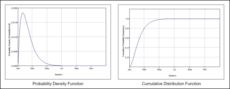
 and Cumulative Distribution (right plot) Functions.")
Stratified Sampling
Stratified sampling in the Hydrologic Sampler changes the distribution of points along the frequency curve sampled. This increases emphasis along a certain portion of the frequency curve, typically the higher magnitude and lower frequency events, reducing the number of total events needed to represent this end of the curve. By default this is turned off and any point along the frequency curve is equally likely to be sampled. With stratified sampling turned on, the probabilities sampled are weighted by a distribution identified by the user. The number of stratified sampling bins is based on the number of years in the lifecycle's analysis period, for example a 50-year analysis period will include 50 bins in the stratification. The width of each bin is used in re-aggregation and summarization of model results. Over the course of generating a set of sampled events in a lifecycle, each bin is sampled in order. Bin-widths are output to each lifecycle's DSS file as a paired data record.
To access the stratified sampling settings, from the Event Sampling tab, click the Edit Stratification Settings button. The Hydrologic Sampling Stratification Setting dialog box opens.
When stratified sampling is turned on (by checking the checkbox to Apply stratification), the user can select a distribution (Gumbel (EV1), Normal, Half-Normal, Exponential, and Uniform), and to which location to apply stratified sampling. The parameters for each distribution is not modifiable by the user. The Smallest exceedance probability of interest setting is used to set the probability at which the final stratification bin should begin.
Note
Stratified Sampling cannot be used with multiple season sampling (e.g., when Two Seasons) is selected. Also, if the Edit Stratification Settings button does not display a checkmark then the Apply stratification checkbox in the Hydrologic Sampling Stratification Setting dialog box was not checked.
