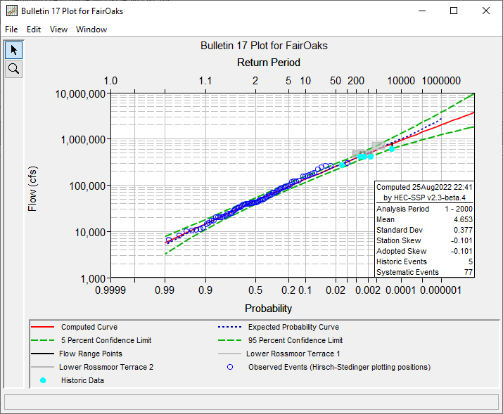
Download PDF
Download page General Settings, Options, and Computations.
General Settings, Options, and Computations
Once the analysis name and flow data set are selected, the user can begin defining the analysis. Six tabs are contained on the Bulletin 17 editor. The tabs are labeled General, Options, EMA Data (which is non-selectable unless the analysis is set to use 17C EMA methods), NEB, Tabular Results, and Variable Time Window Results.
General Settings
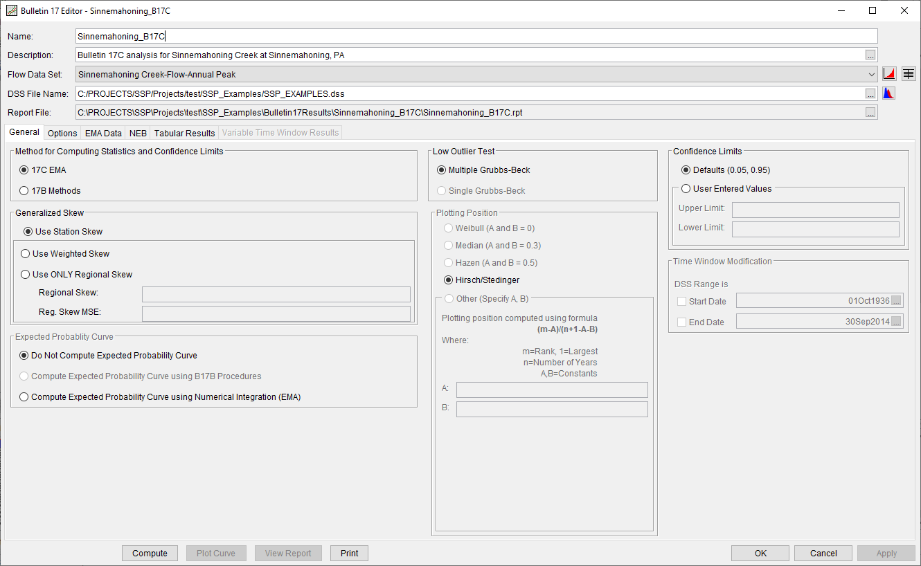
The first tab contains general settings for performing the flow frequency analysis (Figure 1). These settings include:
- Method for Computing Statistics and Confidence Limits
- Generalized Skew
- Expected Probability Curve
- Low Outlier Test
- Plotting Positions
- Confidence Limits
- Time Window Modification
Method for Computing Statistics and Confidence Limits
There are two choices available for computing flow frequency statistics and confidence limits within HEC-SSP as shown in Figure 2: 17C EMA and 17B Methods.

The user is referred to the Bulletin 17C publication for in depth discussions regarding the differences between Bulletin 17B and Bulletin 17C. In general, 17C EMA will provide the same median flow frequency curve as Bulletin 17B methods when there are no historical events/periods and no low outliers included within the analysis. Choosing either 17C EMA or 17B Methods will invoke different options throughout the flow frequency analysis (for instance, choosing the 17C EMA method results in the inability to compute the expected probability curve). When opening a new Bulletin 17 Analysis, the user must select a method for computing statistics and confidence limits before proceeding with the analysis. Until a method is selected, all other options will be inactive.
Generalized Skew
There are three options contained within the generalized skew setting as shown in Figure 3: Use Station Skew, Use Weighted Skew, and Use Regional Skew. The default skew setting is Use Station Skew. With this setting, the skew of the computed curve will be based solely on computing a skew from the data points contained in the data set. No weighting with regional skew will be performed to compute the final skew.
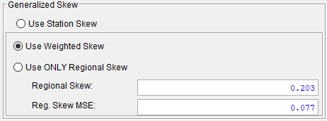
The Use Weighted Skew option requires the user to enter a generalized regional skew and a Mean-Square Error (MSE) of the generalized regional skew. This option weights the computed station skew with the generalized regional skew based upon the inverse of the mean square error in each skew estimate. The equation for performing this weighting can be found in Bulletin 17B (equation 6). If a regional skew is taken from Plate I of Bulletin 17B (the skew map of the United States), the value of MSE = 0.302. Additional estimates of regional skew to be used in peak flow and flow-duration statistical analyses are being developed by the USGS and others; for example, see (Parrett, et al., 2010).
The last generalized skew option is Use Regional Skew. When this option is selected, the user must enter a generalized regional skew and an MSE for that skew. The program will ignore the computed station skew and use only the regional skew.
Expected Probability Curve
This setting has three options as shown in Figure 4: Do Not Compute the Expected Probability Curve, Compute the Expected Probability Curve using B17B Procedures, and Compute Expected Probability Curve Using Numerical Integration (EMA).

The default setting is Do Not Compute the Expected Probability Curve. When using the 17B method to compute statistics and confidence limits, the expected probability curve can be computed using the Compute the Expected Probability Curve using B17B Procedures option. The expected probability curve will be computed using procedures described within Appendix 11 in Bulletin 17B. When using the 17C EMA method to compute statistics and confidence limits, the expected probability curve can be computed using the Compute Expected Probability Curve Using Numerical Integration (EMA) option. The expected probability curve will be computed using procedures described within Margo and Bartles (2022). When an expected probability curve is computed, this curve will be shown in both the result tables and the plots as an additional curve.
The expected probability adjustment is a correction for bias in the computed frequency curve. The bias is caused by uncertainty due to the shortness of the data record. The method of moments estimation of the Log Pearson III parameters produces a median estimate of each frequency curve quantile, and the adjustment changes to a mean (unbiased) estimate, which is different from the median because of the skewness of the uncertainty distribution. The use of the expected probability curve is a policy decision. The expected probability curve is most often used in establishing design flood criteria. When use of the frequency curve includes uncertainty analysis, the expected probability adjustment is made implicitly. Therefore, the computed flood frequency curve without the expected probability adjustment is the curve used in computation of confidence limits, risk analysis, and in obtaining weighted averages of independent estimates of flood frequency discharge (Interagency Advisory Committee on Water Data, 1982).
Low Outlier Test
This option allows the user to choose the test that is performed to identify low-value data points that depart significantly from the trend of the remaining data and inappropriately affect the extreme quantiles in the upper tail of the frequency curve. There are two options for testing low outliers within HEC-SSP as shown in Figure 5: Multiple Grubbs-Beck and Single Grubbs-Beck.

These low-value data points can significantly distort the entire computed flow-frequency curve due to the use of logarithms within both the 17B and 17C EMA methods. These distortions are more severe with the 17C EMA method. As part of the development of the Bulletin 17C methodology, the standard Grubbs-Beck low outlier test was expanded to more successfully identify multiple low outliers (also referred to as potentially influential low floods, or PILFs). Therefore, the only option available when using the 17C EMA method within the Bulletin 17 Analysis is the Multiple Grubbs-Beck test. When low outliers are calculated using the Multiple Grubbs-Beck test, both perception thresholds and flow ranges may be modified within the 17C EMA framework. Example 2 within Appendix C presents an instance where multiple low outliers are identified using the Multiple Grubbs-Beck test and the resulting modification of flow ranges within the 17C EMA framework. When using the 17B methodology, the default test is the Single Grubbs-Beck test.
Plotting Positions
Plotting positions are used for plotting the input flow data set on a probability scale along with the computed frequency curve and confidence limits.
The generalized plotting position equation is:
P=\frac{(m-A)}{(n+1-A-B)}
where m = rank of flood values with the largest equal to 1, n = number of flood peaks in the data set, and A & B = constants dependent on which equation is used (Weibull A and B = 0, Median A and B = 0.3, and Hazen A and B = 0.5). Plotting positions represent estimates of the exceedance probability of each data point (peak flow). Different plotting position formulas can give very different values for the probabilities of the highest and lowest points in the data set.
In both the Bulletin 17B and 17C EMA methodologies, the plotting of data on the graph by a plotting position method is only done as a guide to assist in evaluating the computed curve. The plotting position method selected does not have any impact on the computed curve.
There are five options for computing plotting positions within HEC-SSP as shown on Figure 6: Weibull, Median, Hazen, Hirsch/Stedinger, and user entered coefficients.
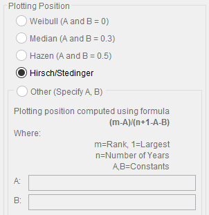
The default method when using the Bulletin 17B method is the Median plotting position formula.
The only method available for computing plotting positions when using the 17C EMA method is Hirsch/Stedinger (Hirsch and Stedinger, 1987). This method sets the A and B coefficients equal to zero. When using 17C EMA methods and the Hirsch/Stedinger plotting position formula, flow data screened as low outliers (a.k.a. Potentially Influential Low Floods) are assigned a plotting position using the Median plotting position formula within HEC-SSP. Also, the user-entered Peak value on the EMA Data tab will be used to determine if a flood represented by a flow interval is above or below a threshold and to rank the flood. For more information, see Margo and Bartles (2022).
Confidence Limits
The computed flow frequency curve is only an estimate of the probability distribution of the parent population. Confidence limits can be used to provide a measure of the uncertainty of the estimated exceedance probability of a selected discharge or a measure of the uncertainty of the discharge at a selected exceedance probability. Confidence limits computed when using the 17C EMA methodology are outlined in Bulletin 17C, Appendix 6. Confidence limits computed when using the 17B methodology are outlined in Bulletin 17B, Appendix 9. Generally speaking, the confidence intervals computed with 17B procedures are less accurate than those computed using the 17C EMA methodology. The 17B methodology neglects the uncertainty in the estimated skew coefficient and does not incorporate historical information. The confidence limits must be entered in decimal form (i.e. 95% = 0.95, and 5% = 0.05). The user has the option to override the default values and enter whatever values they would like for the confidence limits. The options for confidence limits are shown on Figure 7.
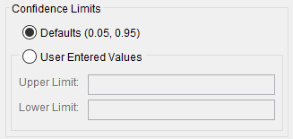
By default, HEC-SSP calculates the 90 percent confidence interval for all flow frequency analyses (i.e. the 5% and 95% percentiles). By comparison, the default confidence interval used within the USGS PeakFQ program is 95% (i.e. 2.5% and 97.5% percentiles) (Veilleux, Cohn, Flynn, Mason, & Hummel, 2013).
Time Window Modification
This option allows the user to narrow the time window used for the analysis. The default is to use all of the annual peak flow data contained in the selected data set. The user can enter either a start date for the analysis, and end date, or both a start and end date as shown in Figure 8. If a start and/or end date are used, they must be dates that are encompassed within the data stored in the selected data set. The date range for the selected data set is shown in the editor just above the Start Date field.

Any dates entered within the Time Window Modification will be ignored when using the 17C EMA Method for Computing Statistics and Confidence Limits. When using 17C EMA, changes to the start and end period must be made within the EMA Data tab.
Options
In addition to the general settings, there are also several options available to the user for modifying the computation of the frequency curves. These options include:
- Low Outlier Threshold
- Variable Time Window
- Historic Period Data
- Output Frequency Ordinates
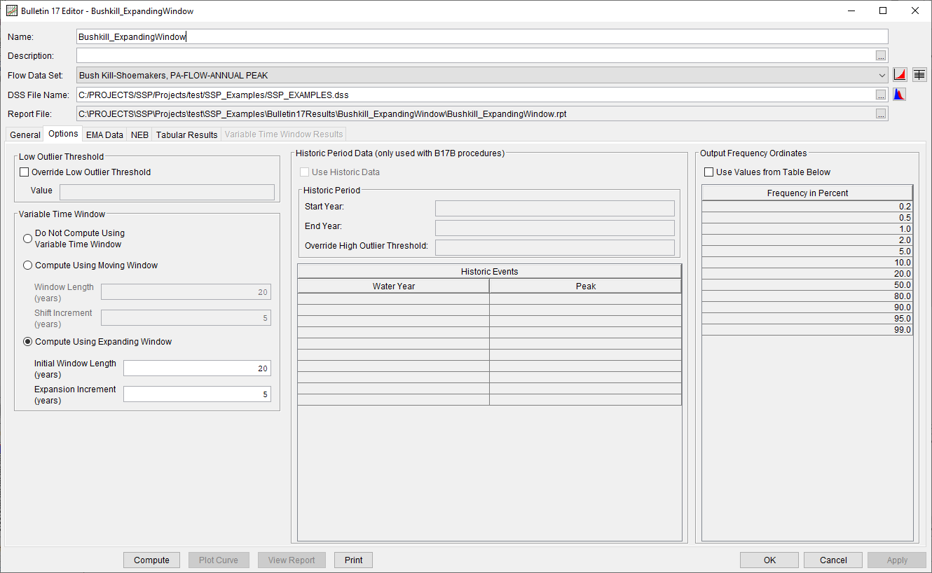
When the Options tab is selected, the Bulletin 17 Editor will appear as shown in Figure 9.
Low Outlier Threshold
The user has the option to enter a value for the low outlier threshold as shown on Figure 10, if desired. If a value is entered for the low outlier threshold, then this value will override the computed value from either the Single or Multiple Grubbs-Beck test. The low outlier threshold cannot be set to a value that would censor more than 50 percent of the values within the data set. To override the computed low outlier threshold, check the box labeled Override Low Outlier Threshold and enter the preferred value.

If the Override Low Outlier Threshold option is NOT used and low outliers are detected, the mean square error (MSE) of the at-site skew coefficient will be computed using equation 6 from Bulletin 17B. However, if the Override Low Outlier Threshold option is used in combination with the 17C EMA Method for Computing Statistics and Confidence Limits, the MSE of the at-site skew coefficient is estimated using a first-order approximation, as described within Cohn, Lane, and Stedinger (2001) and equation 7-27 within Bulletin 17C.
Variable Time Window
This option allows the user to explore how individual flood peaks impact a flow-frequency curve as well as the parameters of the Log Pearson Type III Distribution. There are three options within this panel as shown in Figure 11: Do Not Compute Using Variable Time Window, Compute Using Moving Window, and Compute Using Expanding Window.
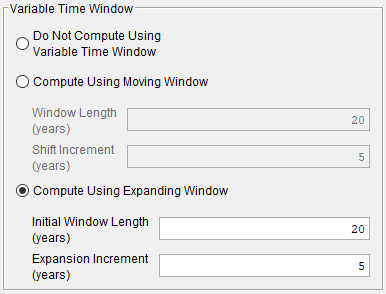
The default setting is Do Not Compute Using Variable Time Window. When using the Compute Using Moving Window option, the input data will be split into multiple analysis windows using the user specified Window Length and Shift Increment, as shown in Figure 12.
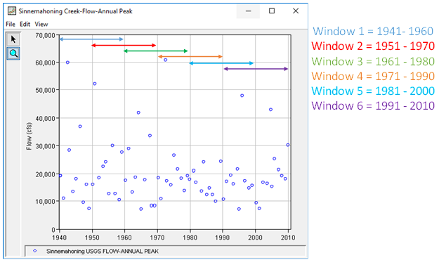
When using the Compute Using Expanding Window option, the input data will be split into multiple analysis windows using the user specified Initial Window Length and Expansion Increment, as shown in Figure 13.
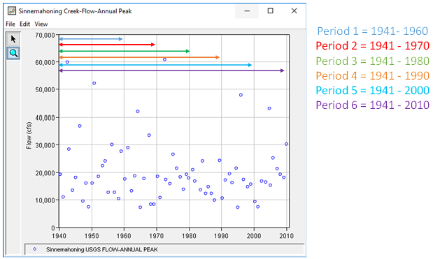
When using the Compute Using Expanding Window option, computations will not be performed until an analysis window is found that contains a number of events that equals or exceeds the specified Initial Window Length.
When either the Compute Using Moving Window or the Compute Using Expanding Window option is used and a compute has successfully completed, the Variable Time Window Results tab will become active and populated with results. Examples demonstrating the use of the Variable Time Window compute option can be found here. A detailed tutorial and guide demonstrating the use of this feature can be found here.
Historic Period Data
This option is only available when using Bulletin 17B procedures. To make use of historic data within the 17C EMA procedures, this information should be entered on the EMA Data tab.
All historic data that provides reliable estimates of flood peaks outside the systematic record should be used in order to improve the estimated flood frequency curve. Flood information of large events outside of the systematic record can often be used to extend the record to a historic period much longer than that of the systematic record. HEC-SSP uses historic data specified in this table as recommended in Bulletin 17B.
To use historic data with Bulletin 17B procedures, check the box labeled Use Historic Data as shown in Figure 14. The user can enter a starting year for the historic period, ending year for a historic period, and a high threshold value to override what is computed. If the user enters a high threshold value, then any value in the systematic record greater than that value will also be treated as a historical flood peak. The user can also enter historic flood peaks that are not contained in the systematic record. This is done in the table at the bottom labeled Historic Flood Peaks. Only one value per water year may be entered and all years must be entered assuming a water year from October 1 through September 30. If a start year is not entered, then the assumed start year is the earliest year of the systematic record and any historical values that have been entered. If an end year is not entered, then the assumed end year is the latest year in the systematic record and any entered historic values.
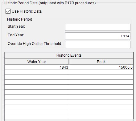
The program treats all data in the data set as systematic data when using Bulletin 17B procedures. If historic events are included in the data set, then the user must define the analysis time window (General tab – Time Window Modification) so that it bounds only the systematic record. Then the user must enter the historic events in the Historic Events table. An example of this application can be found here.
Output Frequency Ordinates
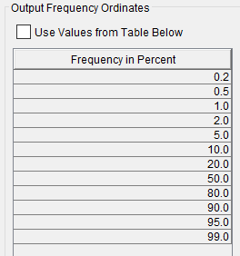
This option (Figure 15) allows the user to change or add to the frequency ordinates for which the resulting frequency curve and confidence limits are computed. The default values listed in percent chance exceedance are 0.2, 0.5, 1, 2, 5, 10, 20, 50, 80, 90, 95, and 99. Check the box next to Use Values from Table below to change or add additional values. Once this box is checked, the user can add/remove rows and edit the frequency values. To add or remove a row from the table, select the row(s), place the mouse over the highlighted row(s) and click the right mouse button. The shortcut menu contains options to Insert Row(s), Append a Row, and Delete Row(s). The program will use the default values, even if they are not contained in the table, when the Use Values from Table below option is not checked. Finally, all values in the table must be between 0 and 100. Note that these values have no impact on the computed frequency curve, but rather only the values of the curve that are reported.
EMA Data
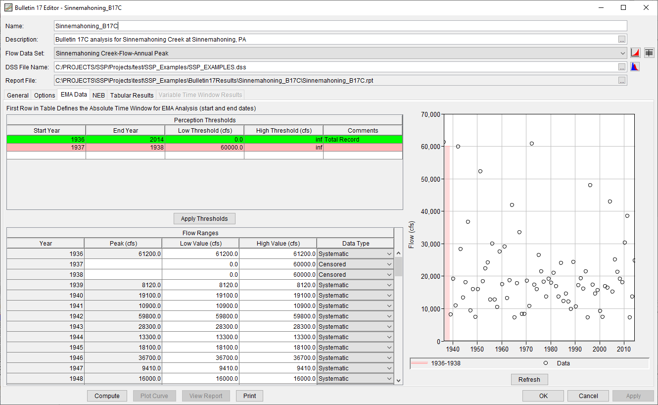
The Bulletin 17C methodology represents a shift in the determination of peak flow frequency and how data is used within peak flow frequency analyses. When using the 17C EMA methodology, additional data is required in order to compute peak flow frequency, confidence intervals, and plotting positions. This new information includes perception thresholds and flow ranges. Every year in the analysis period must have perception thresholds and a flow range specified. The additional data that is required for use within a 17C EMA analysis is accessed/input within the EMA Data tab, as shown in Figure 16.
Perception Thresholds
The EMA procedure introduces the new concept of Perception Thresholds. Perception thresholds define the range of streamflow for which a flood event could have been observed. The inherent assumption and consequence is that any year for which an event was not observed and recorded must have had a peak flow rate outside of (usually below) the perception range.
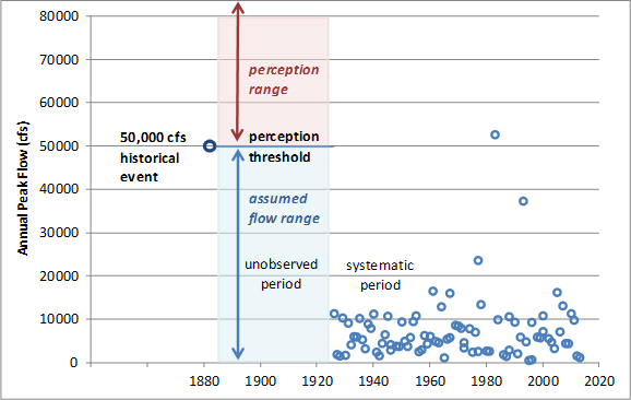
Consider the example of an historical flood in 1882 estimated as 50,000 cfs, and then a gage was installed in 1926. This flood estimate suggests a perception threshold of 50,000 cfs to infinity, because there is evidence that a value as low as 50,000 cfs was noted/perceived (with high water marks, indirect evidence, and/or hydraulic modeling) during the ungaged period. One can further assume that any flow larger than 50,000 cfs would also have been perceived, and so any flow not perceived must have been less than 50,000 cfs. Therefore, for the unobserved period of 1883 to 1925, we assign the complementary flow range of 0 to 50,000 cfs to represent the likely range of peak flows during the unobserved period. The perception threshold and flow range for this hypothetical dataset is shown in Figure 17.
The first row within the Perception Thresholds table will automatically be created to span the entire period of record of the selected Flow Data Set. The start and end year of this first perception threshold can be modified to alter the analysis time frame. This first perception threshold must have a low value of 0 and a high value of infinity. Additional rows within the perception threshold table supersede the rows above, for the specified time frame. However, within HEC-SSP, perception threshold time frames should not overlap one another.
For any missing years in the analysis period, perception thresholds other than zero to infinity must be entered after the first row. The reason for this requirement is that a perception threshold of zero and infinity presumes any flow that occurred could have been observed, implying that unobserved years would not be possible. Therefore, unobserved years must have a perception threshold with either a lower bound greater than zero or an upper bound less than infinity. Most commonly, since very large flows do tend to be observed in some way (as historical events are estimated based on some evidence in the watershed), a lower bound greater than zero is chosen.
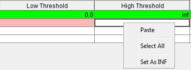
When creating a new row in the Perception Thresholds table, the High Threshold column will automatically be assigned a value of infinity. To manually assign a value of infinity, double left-click to begin editing the desired cell, right-click, and select Set as INF (infinity) as shown in Figure 18.
Use the Comments column to provide a descriptive note to a perception threshold. The use of this column is not required. The comment associated with the first perception threshold will be automatically set to "Total Record". Multiple rows within the Perception Thresholds table can be sorted using chronological order by right-clicking within the table and selecting Sort by Start Year. Similarly, rows can also be inserted or deleted by right-clicking within the table.
When low outliers are detected using the Multiple Grubbs-Beck test, the perception threshold low value for all systematic events will be changed to use the smallest non-screened annual peak flow. Further discussion regarding the impacts of low outliers on perception thresholds along with multiple examples can be found here.
Flow Ranges
The Bulletin 17B methodology limited the use of annual peak flow data to point-value flow estimates or zero flows. The 17C EMA methodology represents each annual peak flow within the analysis period as a range, whether it was observed or not. The flow range for a given year is assumed to be the value itself for an observed value or the complement of the perception threshold for that same year for an unobserved value.
Flow data can be classified within one of three categories: Systematic, Censored, and Historical. This choice is specified in the Data Type column of the Flow Ranges table and can be changed by the user. By default, all flow data contained within the associated Flow Data Set will be set to Systematic while missing years will be set to Censored. Historical data generally refers to flood peaks that occurred outside of the systematic data collection period. Within the USGS NWIS database, a qualification code of "7" will indicate the presence of an historical peak. If this flow data is contained within the associated Flow Data Set, it will be labeled as Systematic by default. The user should change the data type to Historical.
By default, the low and high value for an observed (gaged/systematic) flood event is set equal to the gage estimate. The perception thresholds for these data points are 0 to infinity. However, if there is uncertainty about the flow estimate, the range can expand to represent the possible value(s). Similar to unobserved years in the historical period, if a crest stage gage is unable to estimate flow below a gage base of perhaps 50 cfs, then the perception thresholds would be 50 cfs to infinity, and the associated flow range for an event marked as "limited by gage base" is 0 to 50 cfs, which is set as the complement of the perception thresholds. The flow range for all three data types can be manually altered by the user. Figure 19 demonstrates several possible flow ranges and data types.
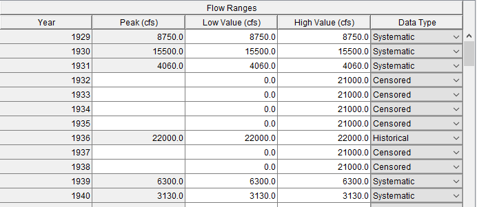
When a flow event is reported as only a high and low value, a value must be entered within the Peak column. This value is used when computing plotting positions for the observed data. Specifically, if the user-specified flow magnitude (as entered within the Peak column) will be used to determined whether the flood is above or below a threshold and to index the flood. More information pertaining to these computations can be found here.
The Apply Thresholds button![]() can be used to automatically fill out the flow range table with the complementary flow ranges. For example, if a perception threshold is specified for a period of missing flow data with a low value of 50,000 cfs and a high value of infinity, the complementary flow range for each missing year would be set to 0 to 50,000 cfs after hitting Apply Thresholds.
can be used to automatically fill out the flow range table with the complementary flow ranges. For example, if a perception threshold is specified for a period of missing flow data with a low value of 50,000 cfs and a high value of infinity, the complementary flow range for each missing year would be set to 0 to 50,000 cfs after hitting Apply Thresholds.
The user should ensure that the peak, low, and high values within the flow range table are appropriate for use before computing the analysis.
The plot within the EMA Data tab (Figure 20) contains the flow values and the complementary Flow Ranges (as determined by the input Perception Thresholds) for the analysis period. The Perception Thresholds themselves are not contained within this figure.
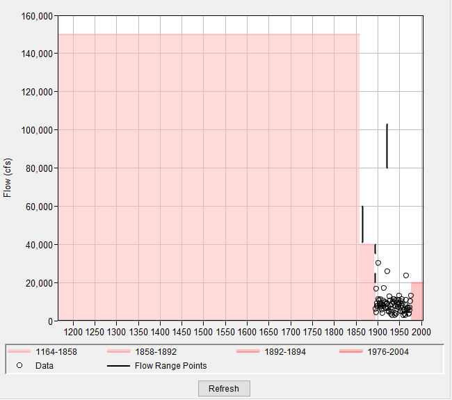
The Refresh button will update the plot if changes are made to either the flow values or Perception Thresholds/Flow Ranges.
The user can double left-click the chart to create a separate window containing the plot. Colors, symbols, and various chart properties can then be edited.
When low outliers are detected using the Multiple Grubbs-Beck test, the high value within the flow range for systematic events will be changed to use the lowest non-screened annual peak flow. Further discussion regarding the impacts of low outliers on flow ranges can be found here.
National Water Information System Qualification Codes
HEC-SSP will import the National Water Information System Qualification (NWIS) annual peak flow and stage qualification/quality codes when available (the program does not import quality codes for daily, instantaneous, and real time data). A description of the quality codes for annual peak flows is contained can be found here and a description of the quality codes for annual peak stages can be found here. These qualification codes can be examined by the user to inform the choice of perception thresholds, flow ranges, and data types.
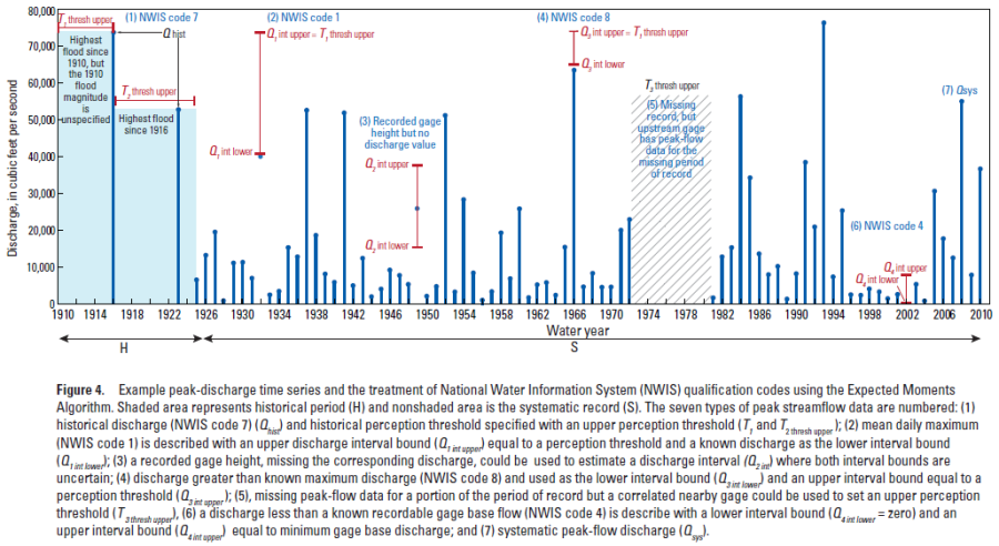
Figure 21 contains an example peak discharge time series and the treatment of the NWIS qualification codes using EMA (Paretti, Kennedy, & Cohn, 2014). Within this example, the shaded area represents the historical period (H) and the non-shaded area represents the systematic record (S). The seven types of peak streamflow data are:
- Historical discharge (NWIS code 7, Qhist) and historical perception threshold specified with an upper perception threshold (T1 and T2 thresh upper).
- Mean daily maximum (NWIS code 1) is described with an upper discharge interval bound (Q1 int upper) equal to a perception threshold and a known discharge as the lower interval bound (Q1 int lower).
- A recorded gage height, missing the corresponding discharge, could be used to estimate a discharge interval (Q2 int) where both interval bounds are uncertain.
- Discharge greater than known maximum discharge (NWIS code 8) and used as the lower interval bound (Q3 int lower) and an upper interval bound equal to a perception threshold (Q3 int upper).
- Missing peak flow data for a portion of the period of record but a correlated nearby gage could be used to set an upper perception threshold (T3 thresh upper).
- A discharge less than a known recordable gage base flow (NWIS code 4) is describable with a lower interval bound (Q4 int lower = zero) and an upper interval bound (Q4 int upper) equal to the minimum gage base discharge.
- Systematic peak flow discharge (Qsys).
NEB
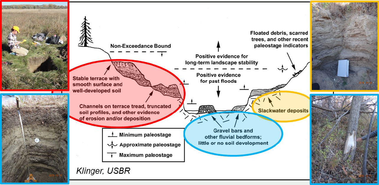
Paleoflood data differs from historical and systematic data in that geologic and physical evidence of past floods provide evidence of paleofloods rather than records based on community memory or referenced by built infrastructure. Paleoflood hydrology focuses on direct evidence of large, rare floods or the absence of such records (England, et al., 2019). Evidence of historic and pre-historic flooding can be provided by flood-related riverine deposits, which are termed Paleostage Indictors (PSI), and/or deposits and landforms that demonstrate an absence of inundation over recent geologic time, which are referred to as Non-Exceedance Bounds (NEB). Examples of PSI and NEB are shown within Figure 22.
Example paleoflood applications using HEC-SSP can be found here.
NEB can be entered on the NEB tab. When the NEB tab is selected, the Bulletin 17 Editor will appear as shown in Figure 23.
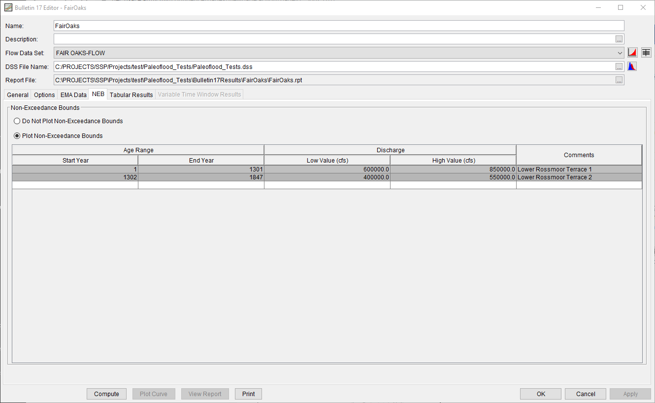
There are two options within the Non-Exceedance Bounds panel: Do Not Plot Non-Exceedance Bounds and Plot Non-Exceedance Bounds. Entries within the Non-Exceedance Bounds table must contain a valid Start Year, End Year, Low Value, and High Value. An optional Comment can be entered as well. The Start and End Year values will be used to compute horizontal bounds for the NEB while the Low and High values will be used to compute vertical bounds for the NEB. The default setting is Do Not Plot Non-Exceedance Bounds. When the Plot Non-Exceedance Bounds option is selected, one or more valid Non-Exceedance Bounds have been entered within the table, and the analysis has been computed, plots of the computed frequency curves will include the entered information, as shown within Figure 24.
