Download PDF
Download page v2.3 Release Notes.
v2.3 Release Notes
Beta released:
Final release:
New Features
Bulletin 17 Analysis
Variable Time Window
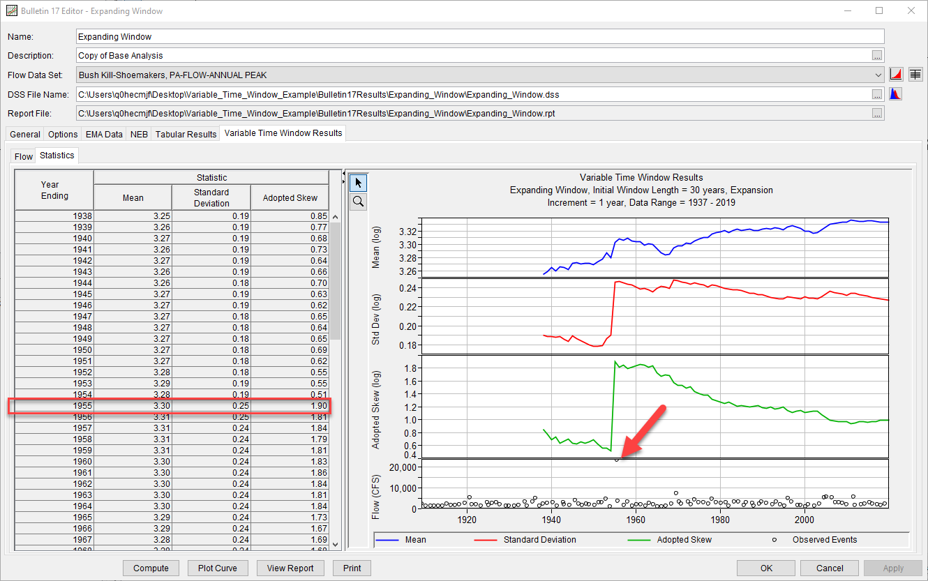
A Variable Time Window option has been added to the Bulletin 17 analysis as a way to explore how statistical parameters or estimates of flow for various annual exceedance probabilities (AEP) change as data is incorporated or removed from consideration. For instance, this feature was used to analyze a record with an extremely large flood when compared to the rest of the data. When the Log Pearson Type III (LPIII) distribution was fit to this data set using increments of 1 year, the inclusion of this extremely large flood was found to cause a large upward shift in the computed mean, standard deviation, and skew, as shown in the following image. A tutorial and guide demonstrating the use of this new feature can be found here.
Plot Summary Panel
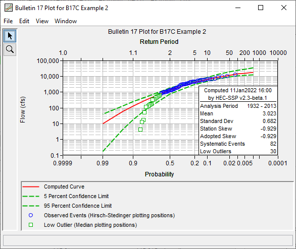
A panel containing summary information has been added to Bulletin 17 plots. Specifically, the date in which the computations were performed, the version of HEC-SSP which was used, analysis period, computed LPIII distribution parameterization (mean, standard devation, station skew, and adopted skew), historic events, systematic events, and low outliers are all shown (when available), as shown in the following image.
Plot Non-Exceedance Bounds
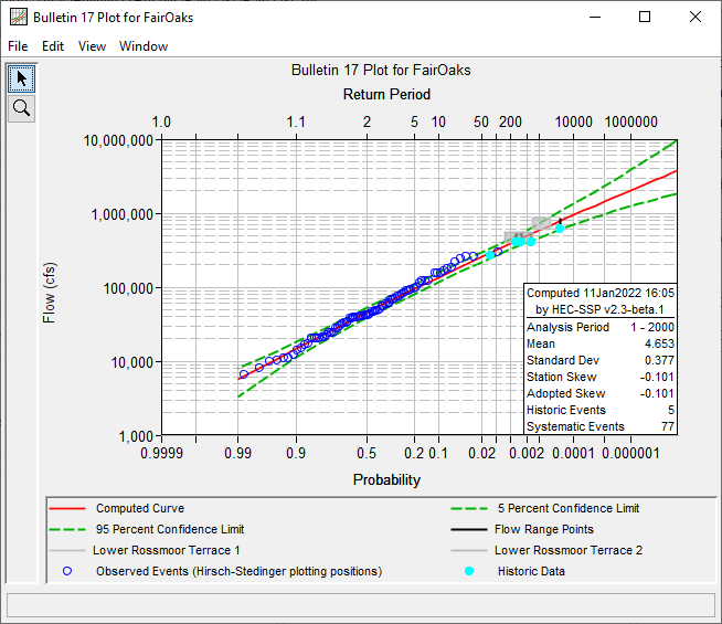
Non-exceedance bounds (NEB) are defined as thresholds above which no flood has been recorded in either historic or pre-historic times. These bounds are commonly derived as part of paleoflood analyses. NEB can now be entered and visualized relative to the parameterized distribution and outputs within a Bulletin 17 analysis, as shown in the following figure.
EMA Data Tab Enhancements
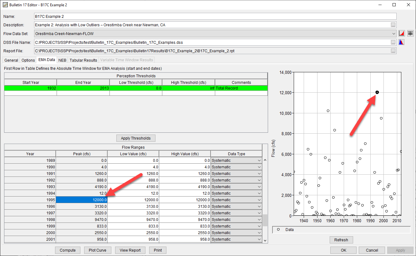
Enhancements to the way in which users enter and interact with perception thresholds and flow ranges on the EMA Data tab have been made within version 2.3. For instance, if a user clicks on a row in the Flow Ranges table, the corresponding event is highlighted/bolded within the plot, as shown in the following figure.
Using Data with Very Old Dates
In previous versions, if the user attempted to use a data set which spanned more than ~4000 years, errors could potentially arise. The underlying DSS library, which handles and interprets the dates associated with values, has been updated to correctly handle dates as old as approximately 10,000,000 years Before Common Era (BCE) and as far into the future as approximately 10,000,000 years. Several example applications using these new capabilities are located here.
Funding partners for the aforementioned Bulletin 17 analysis features included the USACE Fort Worth District, Risk Management Center (RMC), and the USACE General Investigations (GI) program. Initial code implementation was completed by Mark Ackerman, Tevin Youn, Shannon Newbold, Caleb DeChant, and Mike Bartles. Testing was completed by the entire HEC-SSP team. Documentation was completed by Mike Bartles and Matt Fleming.
Bulletin 17C - Expected Moments Algorithm
Multiple enhancements to the Bulletin 17C (B17C) - Expected Moments Algorithm (EMA) and/or features that are intended for use with EMA were made within version 2.3. A presentation containing more details related to these EMA enhancements can be viewed here:
Incorporation of Regional Skew
When using EMA and incorporating regional skew information, previous versions of EMA could erroneously overweight the regional skew information. This overweighting was corrected by implementing Equation 7-10 from Bulletin 17C (England et al, 2019). More information regarding this change along with an example application can be found here.
This correction WILL affect the parameterization of the distribution (i.e. mean, standard deviation, and skew), confidence limits, and quantile variance when incorporating regional skew information. Users are strongly encouraged to update any analyses that incorporated regional skew information to take advantage of these improved techniques.
Effective Record Length
Effective record length (ERL) can be defined as “the number of years of systematic data that would produce the same mean square error [or quantile variance] as a given combination of historical and systematic data” (Cohn and Stedinger, 1986). When all the input data are systematic (i.e. exact), ERL is simply equal to the record length. When some input data consists of flow interval, censored, or regional skew information, ERL is unknown and must be estimated. A variety of stochastic (monte-carlo) based methods exist for the purpose of modeling uncertainty in an analytical flow-frequency curve. These models are commonly used to support a variety of risk-informed decisions. Some examples include the Watershed Analysis Tool (HEC-WAT), Flood Damage Reduction Analysis (HEC-FDA), and Reservoir Frequency Analysis (RMC-RFA). ERL is commonly used as an input parameter to model the uncertainty in the flow-frequency curve using techniques such as the bootstrap (Efron, 1979) or parameter sampling distributions (USACE, 2016). A new ERL computational method was added within version 2.3 which computes a more accurate estimate of ERL when flow interval, censored, and/or regional skew information is included, as shown in the following figure. More information regarding this change along with an example application can be found here.

Plotting Positions for Interval Data
Previous versions of HEC-SSP calculated Hirsch/Stedinger plotting positions for interval data (i.e. low value not equal to the high value) using the geometric mean, or log-average, of the user specified low and high flow values. Specifically, the geometric mean was used to determine if an interval flood was above or below a given threshold and to determine the rank of the flood. Use of the geometric mean lacked transparency and created an interdependence between plotting position and distribution fitting forcing users to make tradeoffs between the two. These situations were most commonly encountered when using paleoflood data which can include evidence (or lack of evidence) of pre-historic floods. The Hirsch/Stedinger plotting position computations have been modified such that the user-specified flow magnitude (as entered within the Peak column) will be used to determined whether the flood is above or below a threshold and to index the flood. More information regarding this change along with an example application can be found here.
This change only affects the computed plotting positions for interval data. The parameterization of the distribution (i.e. mean, standard deviation, and skew), confidence limits, and quantile variance will be unaffected by these changes.
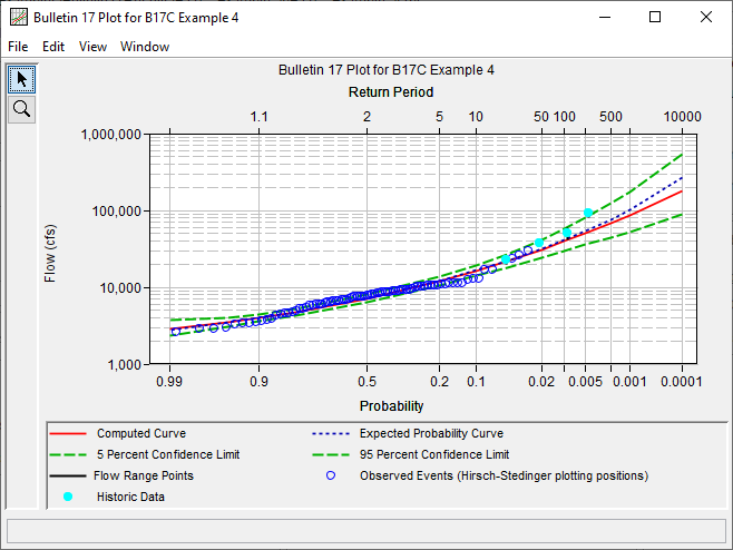
Expected Probability
The expected flow-frequency curve can be described as the expected value of an AEP at a given value of flow and “can serve as a basis for computing the expected return on an investment” (Beard, 1960). The expected flow-frequency curve is the optimal estimator in the context of flood hydrology and should be used to inform decisions (USACE, 1994). The Compute Expected Probability Curve using Numerical Integration option has been added within version 2.3. This option computes numerous confidence intervals to derive an expected probability curve by first inverting the confidence intervals, interpolating them, and finally integrating them. When using the EMA and this option is selected, an expected probability curve will be computed and available for visualization and tabulation, as shown in the following figure.
A webinar detailing these changes can be viewed here:
Check to Ensure Maximum Observation is Within the Supports of the Fitted Distribution
Previously, the supports of the parameterized LPIII distribution were not checked against the largest observation when the skew coefficient was less than 0. This could lead to the use of a parameterized LPIII distribution that could not have produced the largest observation; i.e. for an AEP of ~0, the predicted flow rate is less than the largest observation, which is counterintuitive. Within version 2.3, when the skew coefficient is less than 0, the largest observation is now compared against the support of the fitted distribution. If necessary, the skew coefficient is increased to ensure that the largest observation could have been produced by the fitted distribution.
The previously mentioned enhancements are all available within the Bulletin 17, General Frequency, and Volume Frequency analysis when using EMA. Funding partners for this feature include the USACE GI program and RMC. Initial code implementation was completed by Mark Ackerman, Caleb DeChant, and Mike Bartles. Testing was completed by the entire HEC-SSP team. Documentation was completed by Mike Bartles and Dave Margo.
Data Entry Wizard
Data entry is the first step in any analysis. In order to allow for a more intuitive user experience, a Data Import Wizard was added. This wizard discretizes the steps needed to import data into smaller, more easily accomplished steps, as shown in the following image.

Examples demonstrating the use of this new feature to import data from the USGS website, a Microsoft Excel file, and other data formats can be found here.
Funding partners for this feature include the USACE GI program and RMC. Initial code implementation was completed by Mark Ackerman. Testing was completed by the entire HEC-SSP team. Documentation was completed by Mike Bartles.
Duration Data Filter
A Duration data filter was added which can be accessed by clicking on a data set and selecting Filter. This data filter will create a new data set by averaging the input data over the user-specified duration (in days), as shown in the following figure. Examples demonstrating the use of this new feature can be found here.

Funding partners for this feature include the USACE GI program. Initial code implementation was completed by Stephen Ackerman. Testing and documentation was completed by Mike Bartles.
Year-Over-Year Plot
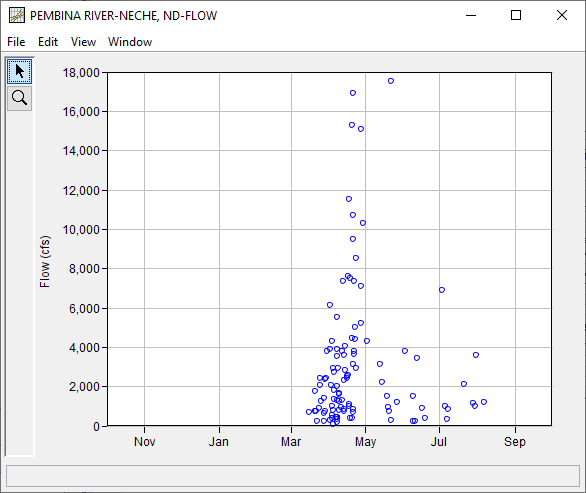
A Year-Over-Year plot, which visualizes all data on a single x-axis that spans a single water year (October 1st - September 30th, January 1st - December 31st, or a user-defined water year), has been added to version 2.3. This plot is available by right clicking on a data set and selecting Year-Over-Year Plot. This type of plot allows for quick analyses of yearly trends. For instance, A Year-Over-Year plot was used to quickly analyze annual maximum streamflow for the Pembina River at Neche, ND. As shown in the following image, the largest and majority of annual maximum floods are produced in March through May. However, several large annual maxima were also produced between May through August which hints at the possibility of multiple flood generating mechanisms.
Funding partners for this feature include the USACE GI program. Initial code implementation was completed by Stephen Ackerman. Testing and documentation was completed by Mike Bartles.
Separate Input and Output DSS Files
Within past versions, a single DSS file was used which contained both input and program outputs/results. Within version 2.3, separate input and output DSS files are created by default. This allows for quicker and more efficient identification of input and output.
Funding partners for this feature include the USACE GI program. Initial code implementation was completed by Mark Ackerman. Testing was completed by the entire HEC-SSP team. Documentation was completed by Mike Bartles.
Plot and Tabulate Data from Editors
Tabulate and plot buttons have been added to all analysis editors within version 2.3. This allows users to more quickly investigate the selected data set(s) within each analysis. An example of this capability within the Bulletin 17 editor is shown in the following image.

Funding partners for this feature include the USACE GI program. Initial code implementation was completed by Mark Ackerman. Testing was completed by the entire HEC-SSP team. Documentation was completed by Mike Bartles.
Correlation Analysis
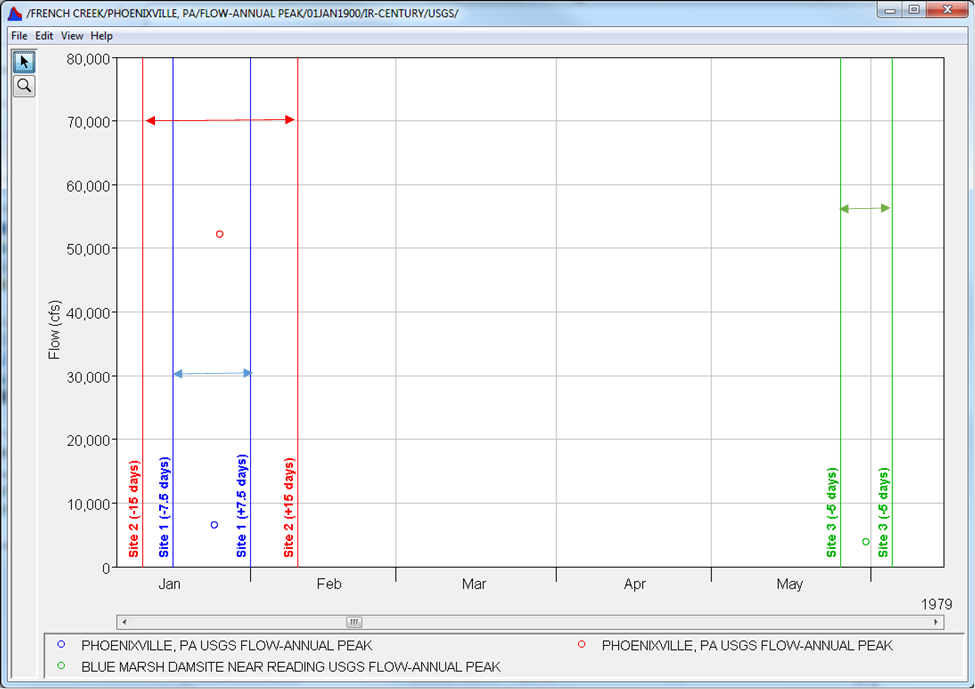
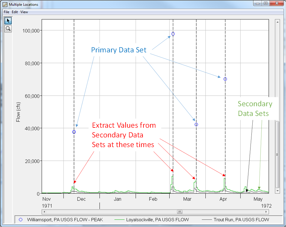
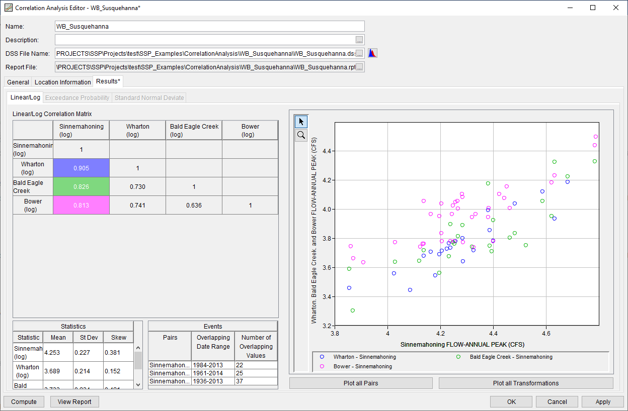
A Correlation analysis was added to version 2.3 in order to compute linear correlation coefficients for multiple pairs of data. Widely varying data types can be used including flow, stage, precipitation, wind speed, and snow water equivalent, amongst others. Three computational methods are available including Coincident Events (which compares the input data to ensure that they correspond to the same “event”), Coincident in Time (which compares a designated "Primary" data set against "Secondary" data in order to extract values for comparison), and Paired Data (which uses the data as defined by the user without any modifications). The following two figures demonstrate how the Coincident Events and Coincident in Time computational methods are used.
Data can be transformed using one or more of the following transformations: Linear, Log, and Exceedance Probability. Output from the Correlation analysis consists of a matrix containing correlation coefficients between each pair of inputs, as shown in the following figure.
Tutorials and Guides demonstrating the use of this new feature can be found here. Funding partners for this feature include the USACE GI program and RMC. Initial code implementation was completed by Mark Ackerman, Tevin Youn, Caleb DeChant, Mike Bartles, and Ryan Cahill. Testing and documentation was completed by Mike Bartles, Matt Fleming, and Ryan Cahill.
Record Extension Analysis
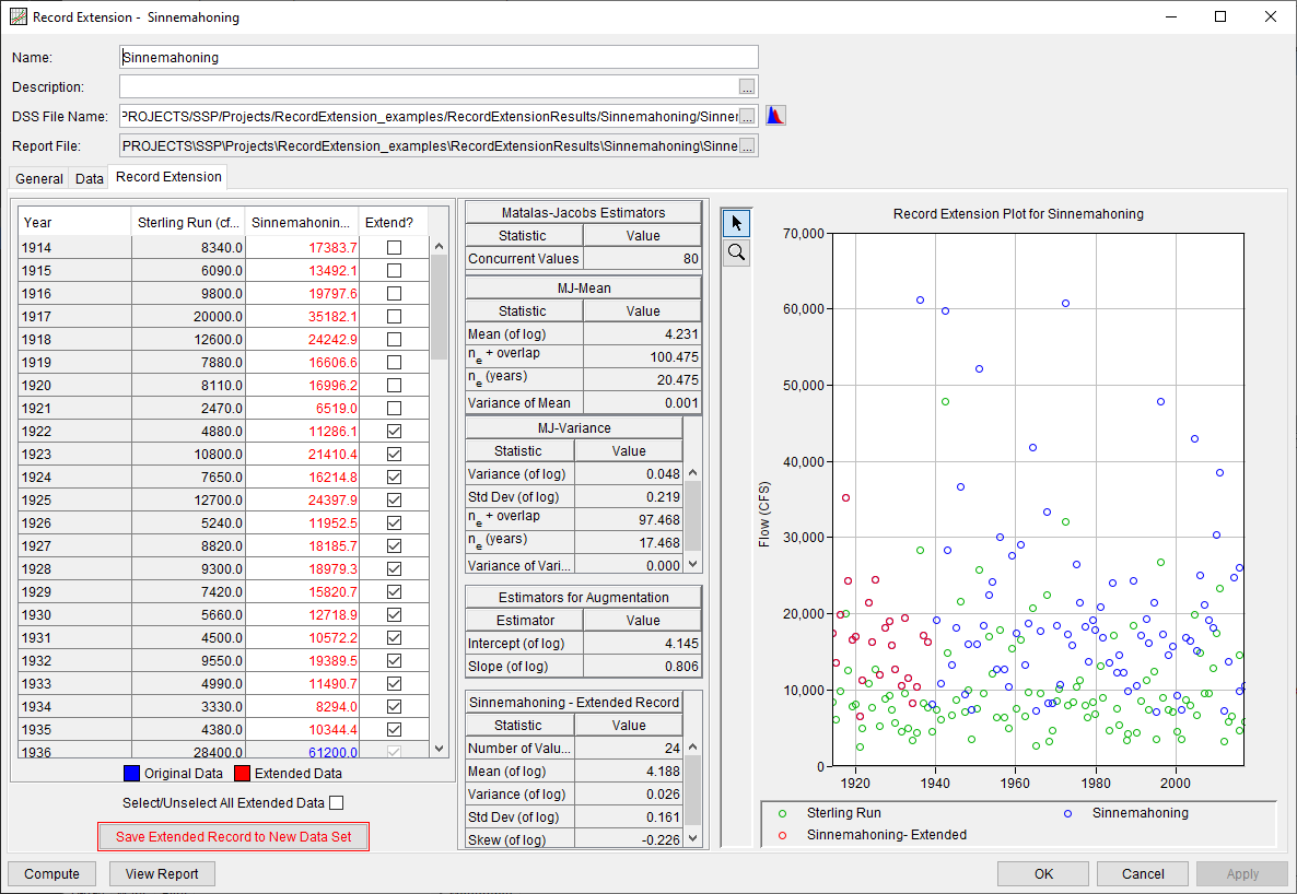
A Record Extension analysis has been added to version 2.3 which allows the user to estimate flows for a location with a short period of record using a location with a longer period of record. Two computational methods, MOVE.1 and MOVE.3 (Bulletin 17C), have been made available to compute an extended record. The MOVE.1 method is documented within Hirsch (1982) while the MOVE.3 (Bulletin 17C) method is documented within Appendix 8 of Bulletin 17C (England, et al., 2019). Both annual maximum series and daily average streamflow can be used within this analysis. Following a successful compute, the extended record is compared alongside the two input data sets on the Record Extension tab, as shown in the following image.
The extended record can then be exported for use within another analysis (e.g. Bulletin 17, Volume Frequency, Duration Analysis, etc).
Multiple tutorials and guides demonstrating the use of this new feature can be found here. Funding partners for this feature include the USACE GI program and RMC. Initial code implementation was completed by Mark Ackerman, Tevin Youn, Caleb DeChant, and Mike Bartles. Testing and documentation was completed by Mike Bartles, Matt Fleming, and Ryan Cahill.
Distribution Fitting Analysis
Analysis Tab
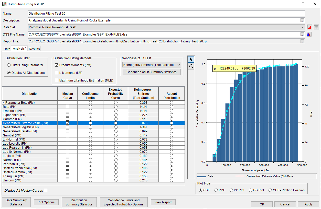
The Distribution Fitting | Analysis tab was modified to allow for better visualization of output as well as simplifying the selection of a chosen distribution. The new Analysis tab is shown in the following image.
Maximum Likelihood Estimation
The Maximum Likelihood Estimation (MLE) fitting method was added to the Distribution Fitting analysis. Now, three methods (Product Moments, Linear Moments, and MLE) are available to fit each analytical distribution, as shown in the following image.
Confidence Limits and Expected Probability Options
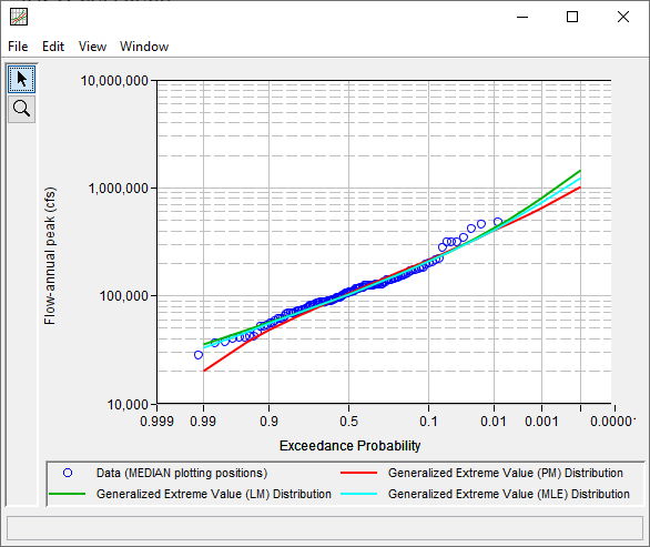
The Bias Corrected and Bias Corrected and Accelerated methods were added to the Distribution Fitting analysis. These methods produce "second-order accurate" confidence limits and expected probability curves for each analytical distribution and fitting method, as shown in the following figure.

These features were funded by the USACE GI program. Initial code implementation of the aforementioned features was completed by Mark Ackerman, Stephen Ackerman, Tevin Youn, Shannon Newbold, Caleb DeChant, and Mike Bartles. Testing was completed by the entire HEC-SSP team. Documentation was completed by Mike Bartles.
HEC-FFA and STATS Legacy Program Importer
HEC-FFA and STATS are two legacy HEC applications which began development in the 1970s and continued through the mid-1990s. As such, numerous studies were completed using these applications up until the initial release of HEC-SSP v1.0 in June 2006. The computational abilities from both programs were incorporated within past versions of HEC-SSP. Version 2.3 introduces a tool to ingest HEC-FFA and STATS study files into an HEC-SSP study. This importer was added in order to transition legacy projects to HEC-SSP.
This feature was funded by the USACE GI program. Initial code implementation was completed by Ryan Ripken. Testing was completed by Mike Bartles and Matt Fleming. Documentation was completed by Mike Bartles.
Bugs Fixed
The following bugs were present in previous versions and have been fixed within version 2.3.
Computing a Bulletin 17 Analysis with More Than One Value Per Year
If the user attempted to compute a Bulletin 17 analysis using B17C procedures and more than one value per water year (i.e. 01Oct – 30Sep) was contained within the selected flow dataset, a null pointer exception was thrown and the compute halted. While the compute was correctly halted, a more descriptive error message should have been presented to the user. An improved error message has been added to inform the user of the problem. Users are encouraged to utilize the General Frequency analysis (which also allows for the use of EMA) to fit a Log Pearson Type III distribution to an annual maximum series where events are demarcated using a water year other than 01Oct – 30Sep.
Flow Ranges Table Cleared within General Frequency Analysis
Upon opening a HEC-SSP study and navigating to the EMA Data tab within an existing General Frequency analysis, the Flow Ranges table was cleared for rows that used the Censored data type. This issue has been rectified within version 2.3.
Infinity to Infinity Perception Thresholds within General Frequency Analysis
[inf – inf] perception thresholds were not allowed within General Frequency and Volume Frequency analyses. This has been fixed within version 2.3.
Analyses with a Blank File Name
Within previous versions, loading analyses with blank file names (e.g. "[blank].da") could cause the program to freeze and/or act inappropriately. Within version 2.3, if analyses with blank file names are encountered, they will be removed from the HEC-SSP project and a warning message will be shown to the user.
Exception Plotting Results for Analyses That Haven't Been Previously Computed
When attempting to plot results for analyses that haven't been computed, an exception was thrown in previous versions. Within version 2.3, if analyses don't have results and the user attempts to plot, the exception is suppressed and no results will be shown.
Balanced Hydrograph Analysis Incorrect Imported Data Out Of Date Message
A message warning users that imported data was out of date was being incorrectly shown within the Balanced Hydrograph analysis editor whenever any Bulletin 17, General Frequency, or Volume Frequency analysis was computed. Now, this message will only be shown when linked Bulletin 17, General Frequency, or Volume Frequency analyses are computed.
Peaks Over Threshold Filtering
In some instances when using the Peaks Over Threshold Data Filter with an optional Defined Threshold Value, Differential of Peak, or Percent of Peak, peaks were being rejected even though they were valid. In other instances, the last peak in a cluster of peaks was being erroneously retained. These issues within the Peaks Over Threshold Data Filter have been removed such that only the correct peaks that meet all defined criteria will be retained.
Copying/Pasting from Perception Thresholds Table
When copying data from the Perception Thresholds table, the data would be inverted when pasted into applications such as Microsoft Excel. Now, when copying from a Perception Thresholds table within either a Bulletin 17, General Frequency, or Volume Frequency analysis, the data will be copied to the clipboard appropriately.
Creating an Empty Analysis
Within previous versions, an empty analysis could be created when the user clicked the cancel button within an analysis editor. Within version 2.3, no empty analyses can be created.
Beta Releases
Release | Date | Features | Bug Fixes |
|---|---|---|---|
| beta.1 |
|
| |
| beta.2 |
|
|
|
| beta.3 |
|
|
|
| beta.4 |
|
|
|
| beta.5 |
|
|
|
| Final Release |
|
|