PDF
Download PDF
Download page New Features.
New Features
HEC-RAS 6.4 Released
Major Features
- 1D Unsteady Flow Encroachment Analysis
1D Unsteady flow encroachment analysis provides capability for the 5 traditional methods of analysis as well as integrating Encroachment Regions for limiting the water surface in the floodplain fringe. It is intended that users can perform floodway encroachment analysis on 1D, 2D, or combined 1D/2D models with a mix of encroachment methods. However, it is anticipated that the final runs will be performed using Encroachment Regions.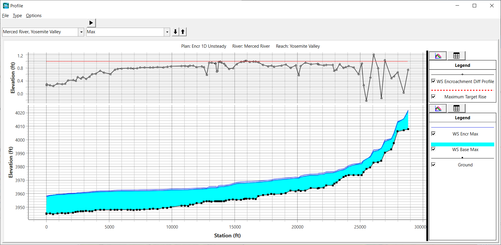
- 2D Unsteady Flow Encroachment Analysis
2D Unsteady flow encroachment analysis provides the capability to perform encroachment analysis on 2D models. The tools and methods in HEC-RAS allow the user to create Encroachment Regions which are applied as a Terrain Modification which fills the floodplain fringe thereby allowing the reuse of the same 2D mesh for a Base geometry and the Encroached run. Tools are available to automatically generate Encroachment Regions based on mapping results from previous (base) runs.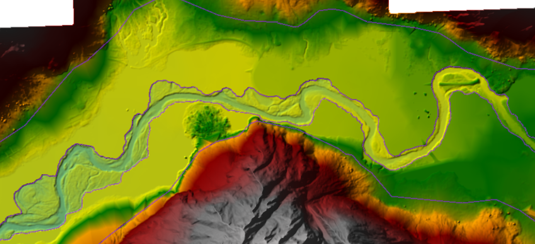
- Flow Optimization
Flow Hydrograph Optimization in HEC-RAS is an automated tool that allows the user to specify a Reference Location for the model to monitor either Stage or Flow and perform adjustment to the inflow hydrographs to hit a Target Value specified by the user. This option may to be used to identify flow requirements by scaling a predefined hydrograph (or set of hydrographs) by a specified Flow Ratio for flows coming into a reservoir or in a river at a levee location in order to bring the stage up to a specific height (to breach a structure or keep water from over-topping).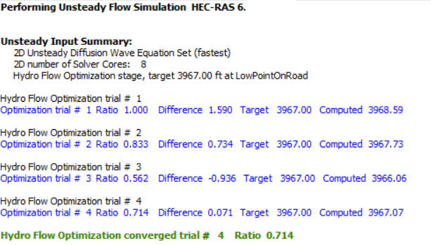
- Atmospheric Pressure
In order to support modeling of compound flooding in coastal areas, HEC-RAS has added spatially variable atmospheric pressure forcing to all flow solvers. Atmospheric pressure can be specified at Meteorological Stations, DSS grids, or GDAL raster files. The atmospheric pressure input is very similar to how other spatially variable meteorological data is entered (see figure below).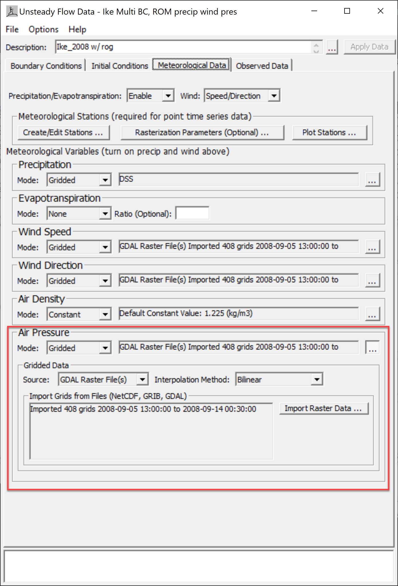
Below is an example grid of atmospheric pressure forcing in the Dickinson Bayou, in Galveston Bay, Texas.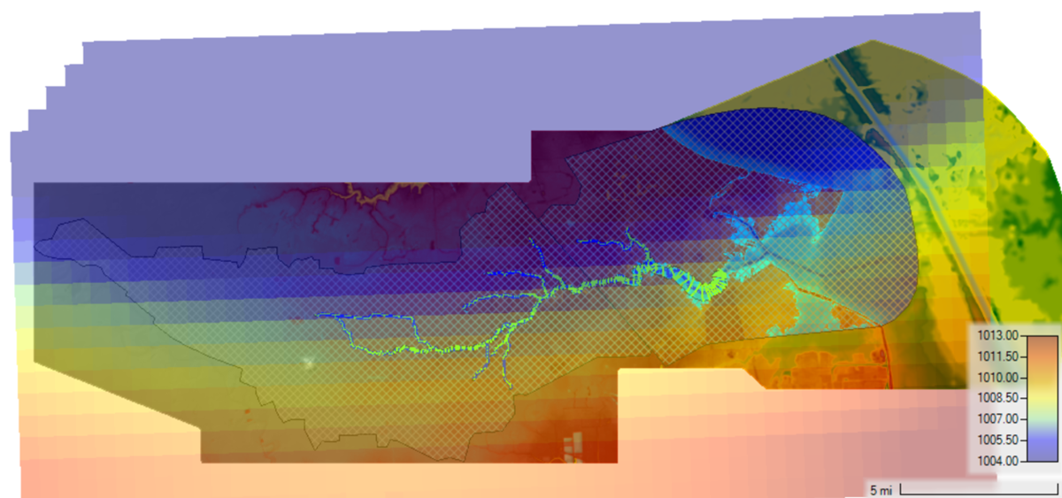
- Render Mode Improvements
An additional interpolation scheme is available in 6.4. A simple Sloping method using 2D cell corners for interpolation has been re-introduced.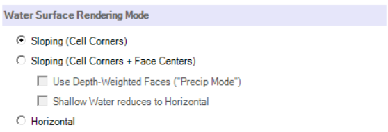
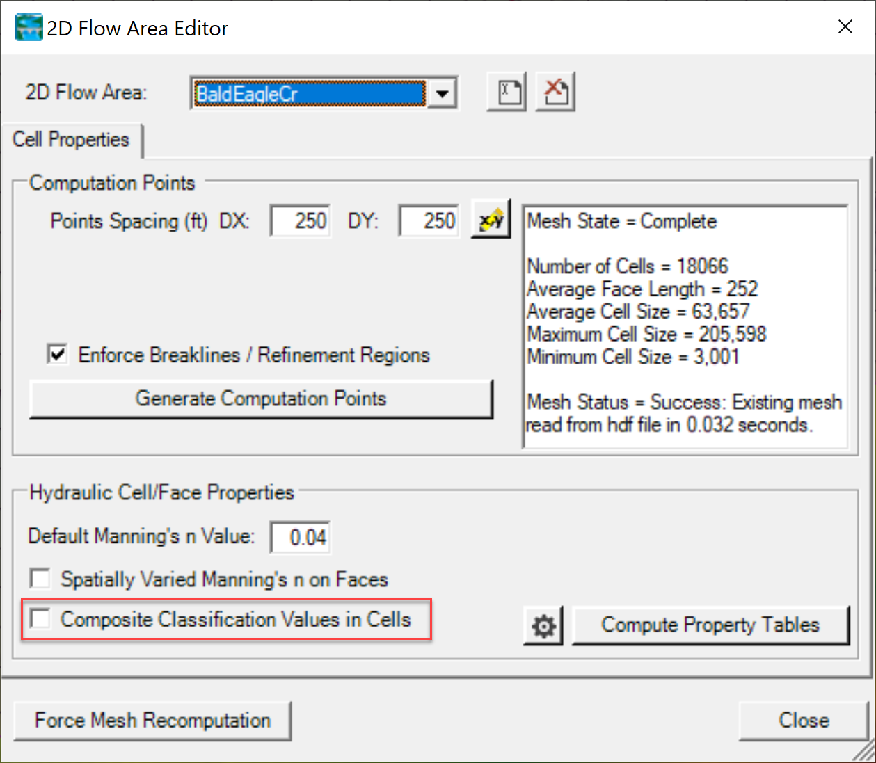
- Composite Land Classification Values - A new feature for land classification values allows to be spatially composited over each cell rather than a single point value at the center.
- Reference Area Query and Volume Time Series (Video)
Users can add a "Reference Polygon" to Mapper (like a reference line or point) and aggregate or average results for all the cells in that area. This will be useful for computing the total volume associated with a group of cells, an average velocity, or a total bed change in a sediment model (summing erosion and deposition to compute the net bed change).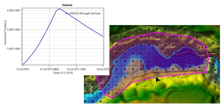
- Fixed Bed 2D Sediment Transport Analysis: (Capacity Only and Concentration Only)
The 2D sediment model now supports "fixed bed" sediment modeling which simplifies sediment analysis substantially and offers "incremental complexity" sediment analyses between a simple, hydraulic, shear stress analysis and a full mobile bed model. The "Capacity Only" tool evaluates the transport capacity associated with each cell and cell face at each flow without the feedbacks (or computational expense) of erosion or deposition. The result below used the RASter calculator to compute the capacity with and without the evaluated structures, generating spatial and cross section analysis on how these structures will affect sediment transport through this reach.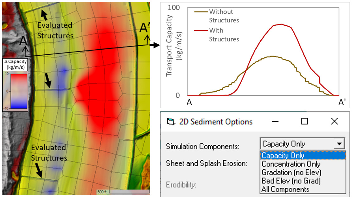
- Raster Export Options
All map results have export options to write information to a file. Map results can be exported to a raster dataset (GeoTiff) or to vector contours. The various export options discussed below are available by right-click on the map layer and choosing from the Export Layer menu items.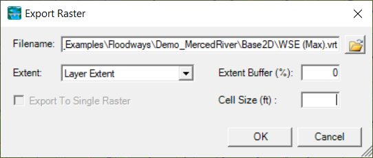
Minor Improvements
- Automated Annual Sediment Load Computation (and Sedigraph) in the Sediment Rating Curve Calculator (Video)
The HEC-RAS Sediment Rating Curve Analysis Calculator will automatically pull the flow data (blue line below) from a USGS gage and use the rating curve developed with the sediment data to develop a full time series of sediment load (brown line below), plotting it with the observed sediment loads (black dots below). Then the tool will annualize these loads, to report an average annual sediment load (in tons/year) to help users develop their sediment budget.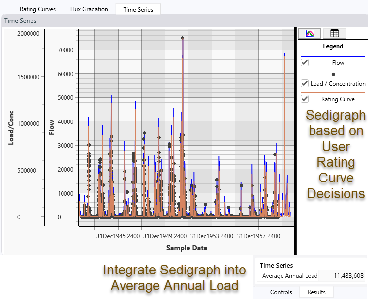
- Large Woody Debris (LWD) Terrain Modification (Video)
Version 6.4 includes a LWD terrain modification that allows users to add tree with a separate root wad diameter to the terrain. The trees are compound shapes, combining two rectangles or a rectangle and a triangle and can be placed horizontally (above a specified base elevation - which can be partially buried) or added to the terrain along a slope.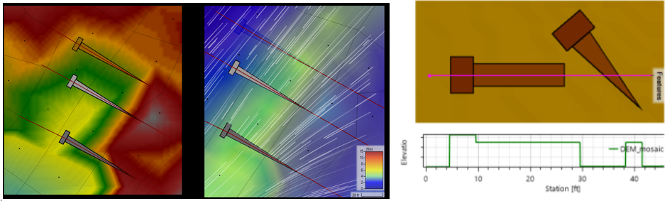
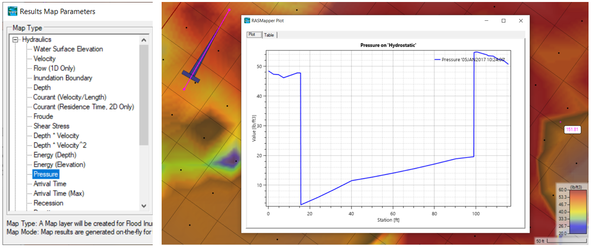
- Hydrostatic Result Map (For LWD Stability Analysis)
- LOESS Local Regression for Sediment Rating Curves (Video - 2nd half)
New tool in the Sediment Rating Curve Calculator in the Hydraulic Design Toolbox applies a non-parametric, local regression using the LOESS method. This method can compute an "optimal span" (the local moving "window" of data that the model uses - higher spans tend to smooth data) and plot analytics on the different span ranges. But users can choose any span (0-1) to plot a local regression model and identify local trends in their data.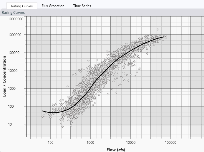
- New Cohesive Methods in 2D Sediment
- Equilibrium Shear Stress Range
- Non-Linear Excess Shear
The 2D sediment model added two alternate cohesive methods to make cohesive modeling more flexible. (Note: We also updated the documentation on the dimensionless vs dimensional (Kd vs M) excess shear equations work and interact).
- Convergence Messaging for 2D Sediment
The 2D Sediment model now writes orange messages if the model reaches max iterations during a sediment solution time step. These messages only tell users if a cell has gone to max iterations, not which cell or how bad it is. But we have added detailed documentation on how to request and interpret the computational level output file that helps users identify the offending cells and evaluate the magnitude of the problem.
- Residual Plots for Piecewise Linear Sediment Regression
Version 6.4 includes a residual plot with the piecewise linear sediment rating curve algorithm to help users decide if a local-residual minimum (e.g. in the more sensitive moderate-to-high flow region of the curve) would be more appropriate than the global minimum.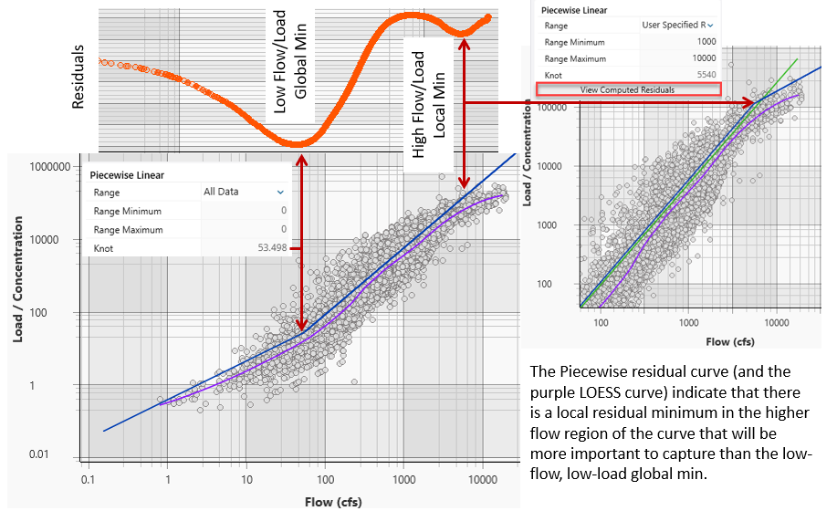
Tutorials
- 1D Unsteady Flow Encroachment Analysis
- Flow Hydrograph Optimization
- 2D Rules Example
- Expedited Debris Flow Tutorial
- 2D Sediment
- Parameter Summary Guide (which parameters do we recommend changing and within what range) and
- Runtime Optimization Guide (how to make the model run faster)
HEC-RAS Publications
Sediment Rating Curve Calculator (SEDHYD)
Example Dam Removal Sediment Model in HEC-RAS (SEDHYD)
Mud and Debris Modeling (SEDHYD)
Two Example Debris Flow Models in HEC-RAS (SEDHYD)
Sediment Modeling Failure Modes and Best Practices (SEDHYD)