HEC-GeoEFM is used in the spatial analyses phase of the HEC-EFM process to help manage and assess spatial data layers and to quantify the amount, quality, connectivity, and functionality of ecological habitats generated by different
water management or ecosystem restoration scenarios.
Contents:
Habitat Areas
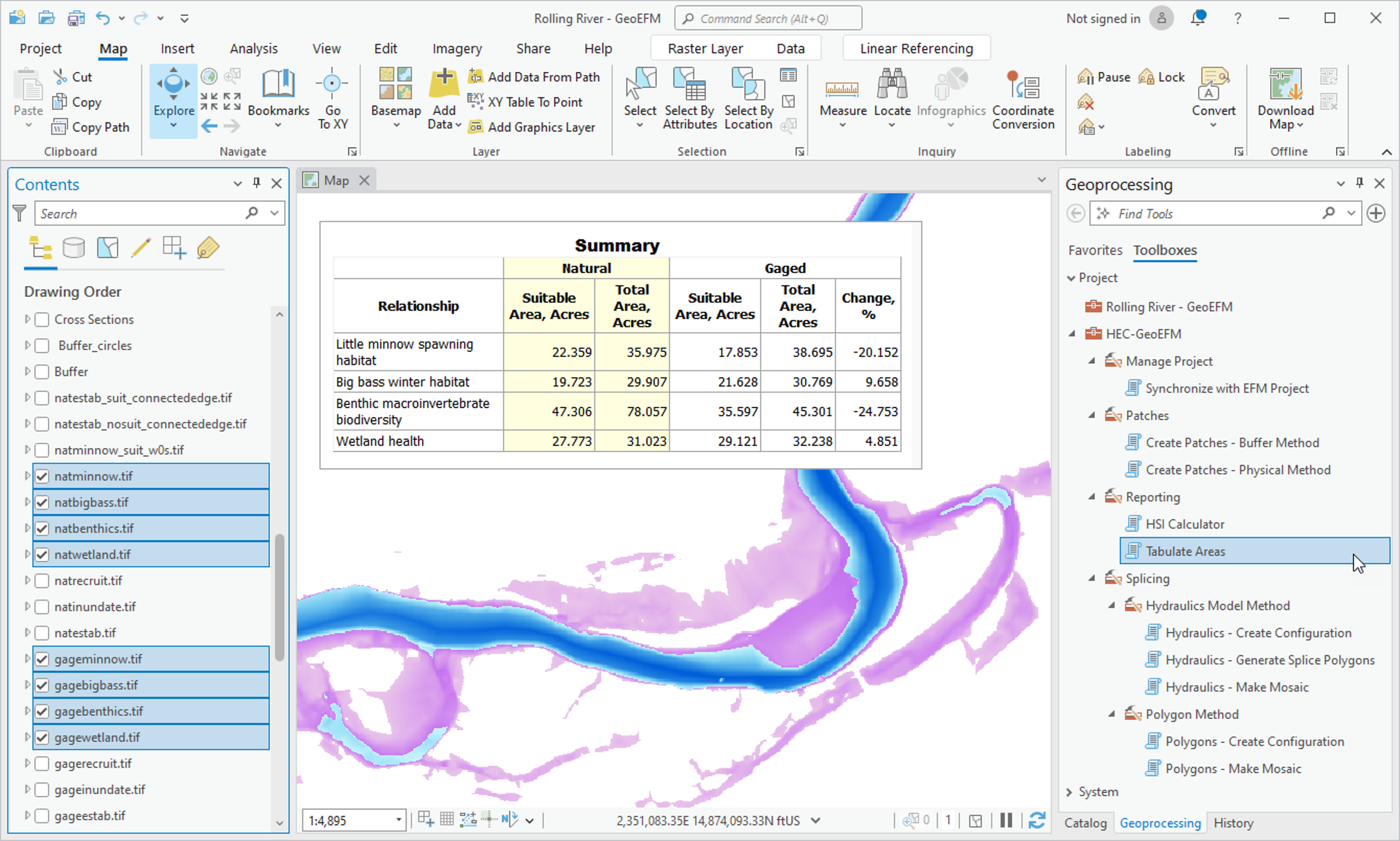
HEC-GeoEFM has a tabulate tool that allows users to compute, report, and archive total habitat areas. Options are provided for selecting the desired flow regimes and relationships, output units, and mode of
comparison for multiple flow regimes.
Back to the top
Habitat Quality
GeoEFM allows users to add, copy, rename, and delete Habitat Suitability Indices (HSIs). HSIs relate a variable such as water depth or velocity to a measure of habitat quality that ranges from 0 (wholly
unsuitable) to 1 (perfectly suitable). HSIs are commonly used in ecological modeling, including model applications for habitat mapping.
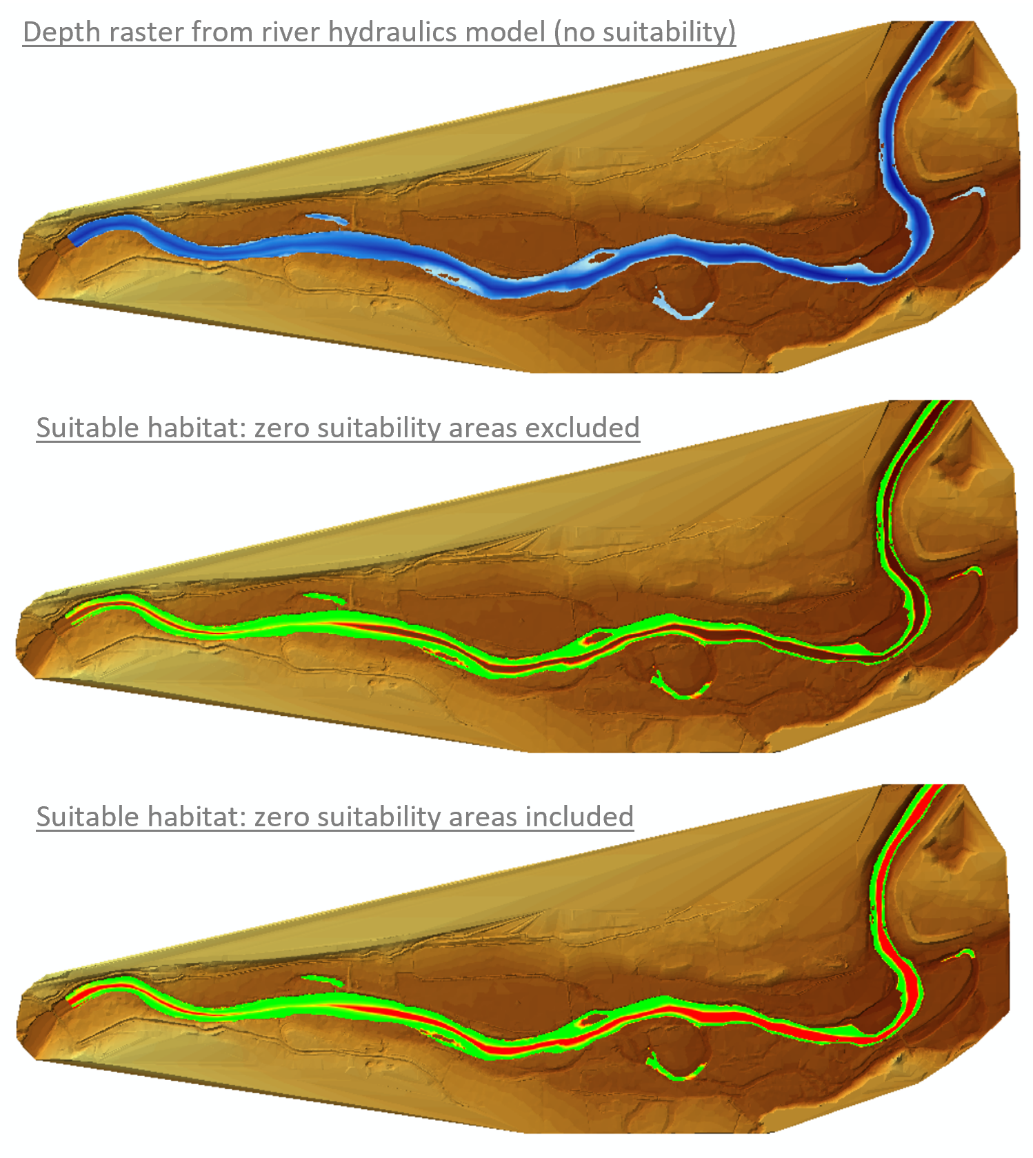
HSIs are applied to raster layers via GeoEFM HSI calculators. For example, the image below shows a HSI (Little Minnow – Depth) being applied to a raster of water depths (nat-minnow) to generate a suitability
raster. An option is provided that allows the users to pick whether to exclude (checked) or include (unchecked) zero suitability areas from the output raster.
Habitat quality considerations have also been integrated into GeoEFM tools related to habitat area, connectivity, and functionality.
Back to the top
Habitat Connectivity
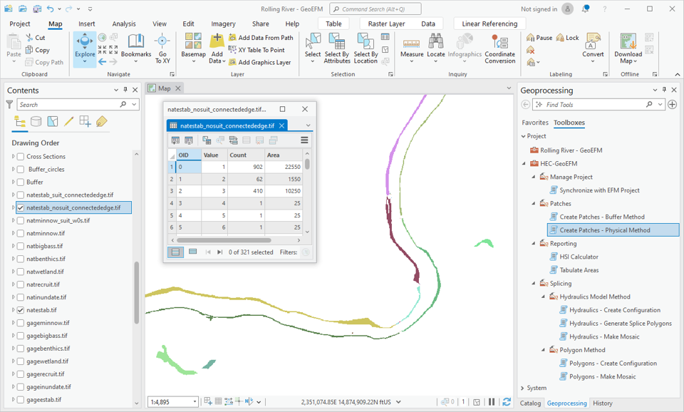
GeoEFM’s Patch Analysis tool is used to analyze how different patches of habitat are connected. The Physical connectivity option allows users to group raster habitat cells into connected patches.
Output includes the number and size of patches that occur within user-defined areas of interest.
Back to the top
Habitat Functionality
Ecological concepts like habitat corridors, fragmentation, and functionality can be explored using the GeoEFM nearest neighbor and buffer methods, both of which parse habitat into the unit habitat areas (i.e., patches)
that would support individuals or groups of individuals within a population.
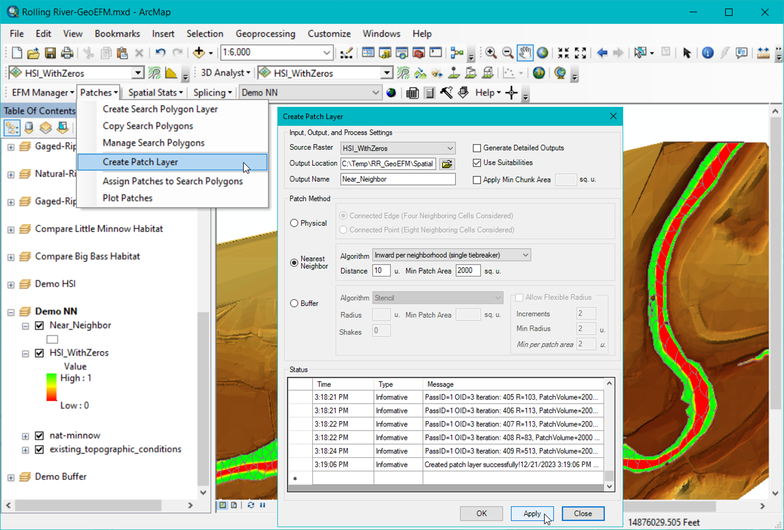
Nearest neighbor is most applicable to gregarious communities that are not strongly territorial. The figure below shows nearest neighbor patch results for a raster processed with consideration of habitat quality.
Larger patches occur in the poorest habitat because more total area is required to meet the user-specified area (suitable) required to make a patch. Please note that nearest neighbor is available only in GeoEFM 2.0.
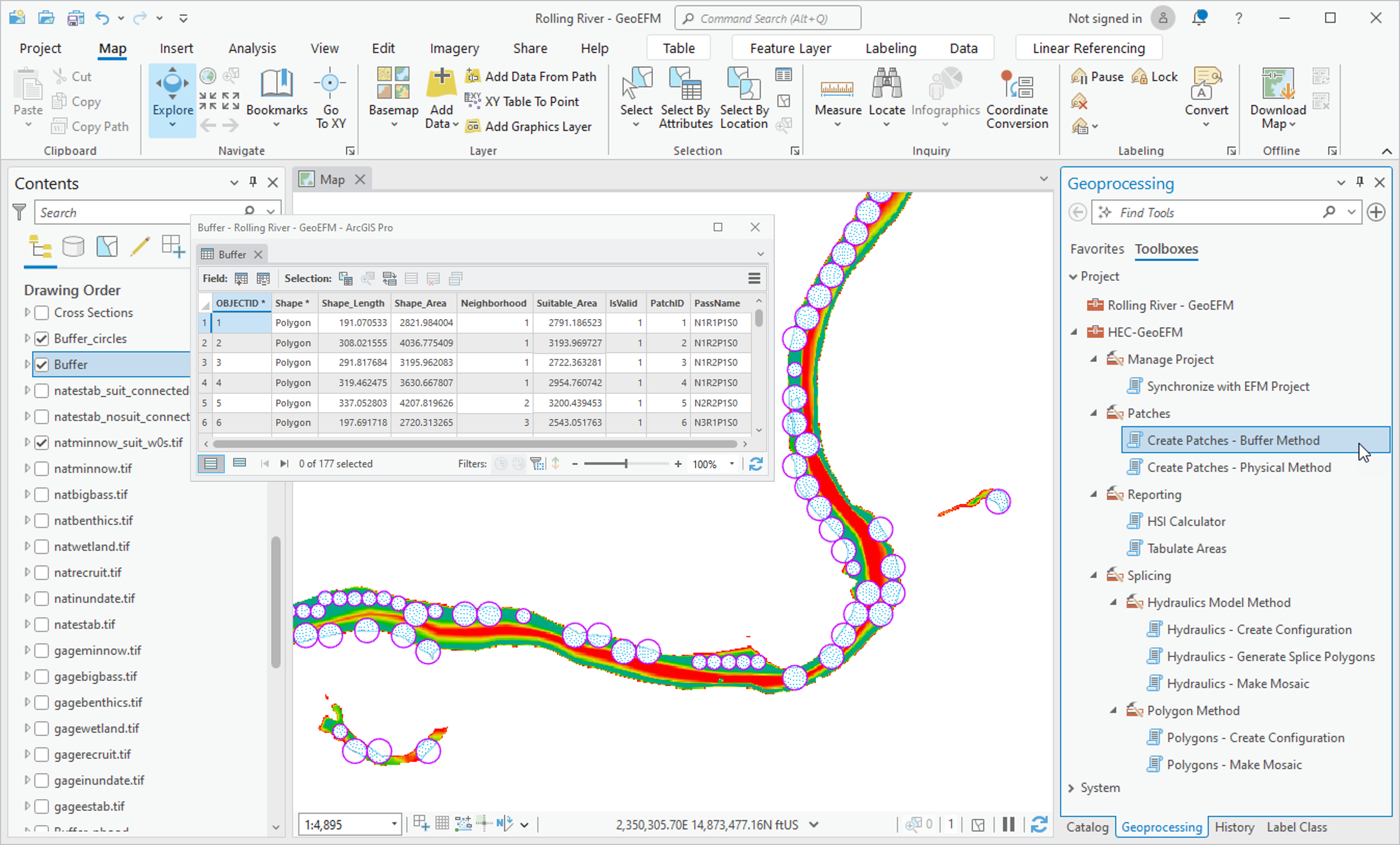
Buffer is most applicable to territorial communities that inhabit or utilize or protect an area for one or more of their life stages such as nesting. The figure below shows buffer patch results for a raster processed
with consideration of habitat quality. Patches cut with the larger radius tend to occur in the poorest or sparsest habitat because the larger radius was needed to meet the user-specified area required to make a patch.
Back to the top
Habitat Mosaics
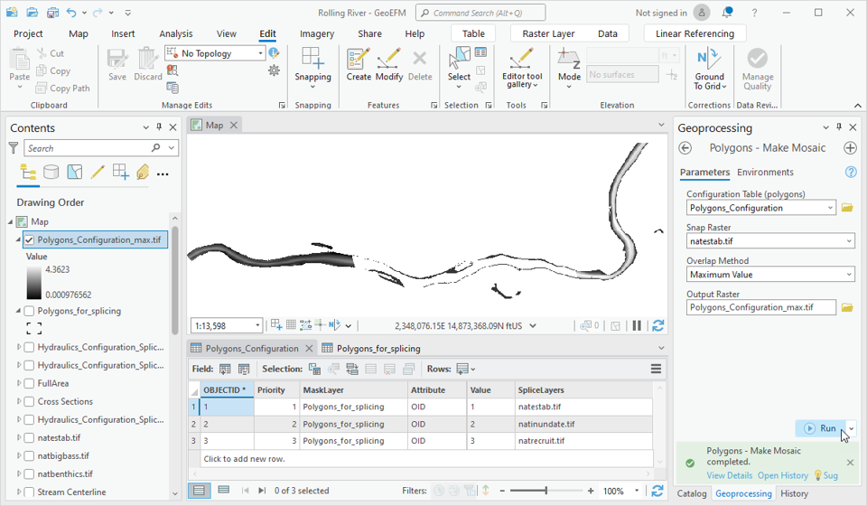
In aquatic systems, habitat for a species or species life stage is often spatially dispersed within the system’s connected waters. In GeoEFM, habitat mosaics can be made such that habitat in different river reaches and
connected waters are spliced into a single habitat map. The basic process for splicing is to associate habitat layers with spatial areas and then merge the layers accordingly. There are three splicing methods:
Polygon, raster, and hydraulic model. Choice of method is controlled by the user. Options are provided to handle areas of overlap. The figure below shows a polygon splice and resulting mosaic.
Back to the top
Spatial Statistics
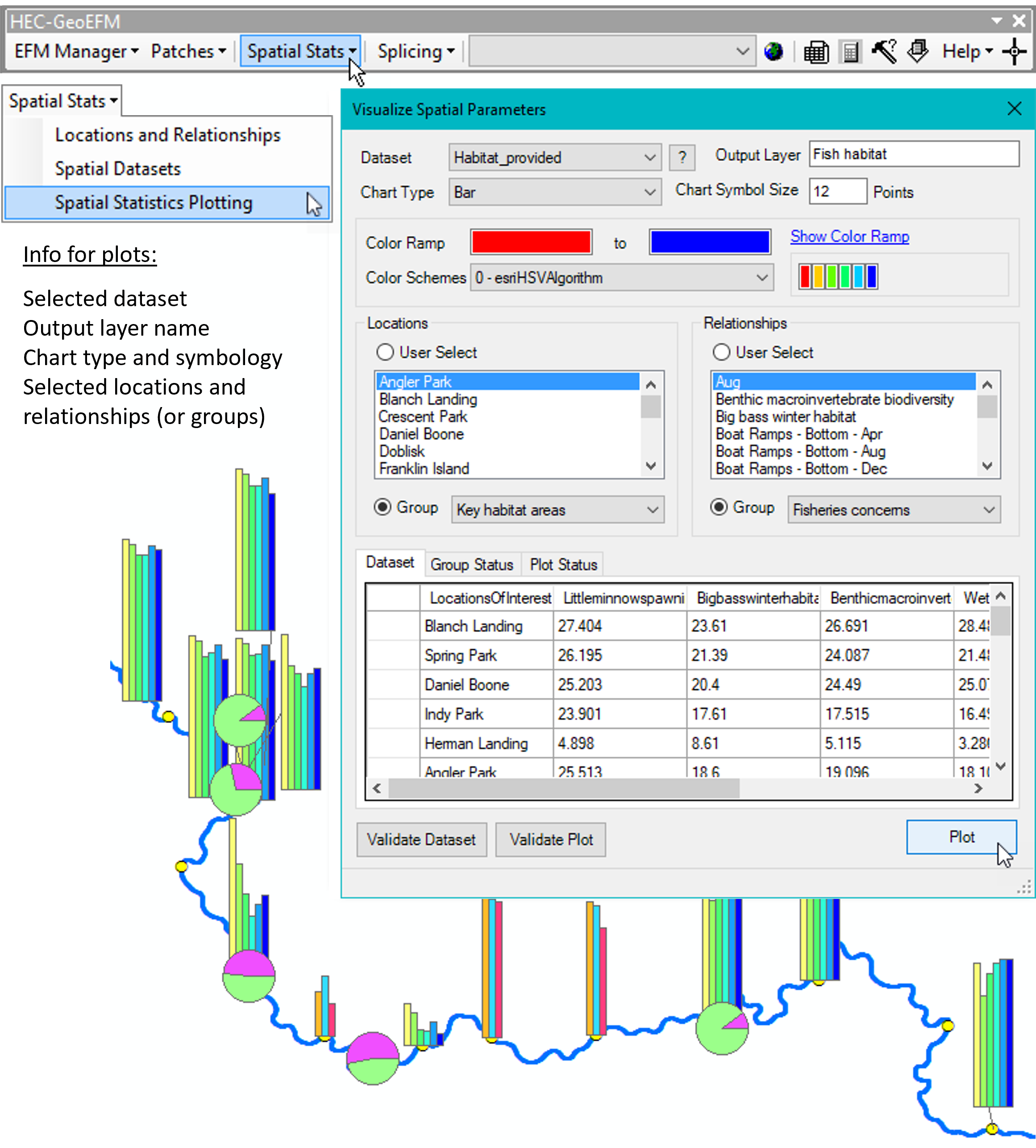
GeoEFM can be used to display statistical results spatially. This is a different workflow than habitat mapping. Instead, statistical results are associated with locations and then plotted. Information for plotting are
stored in three basic data tables: Locations, relationships, and datasets. After those tables are populated, data values may be viewed as spatially distributed bar, pie, and stacked chart graphics. Please note that spatial
statistics is available only in GeoEFM 2.0.
Back to the top