Download PDF
Download page Pre & Post Wildfire Hydrology Modeling with HEC-HMS Procedure.
Pre & Post Wildfire Hydrology Modeling with HEC-HMS Procedure
Last Modified: 2023-02-23 06:27:20.29
This tutorial demonstrates a process to configure and calibrate an HEC-HMS model for pre and post wildfire modeling.
Software Version
HEC-HMS version 4.11 was used to develop this tutorial.
Introduction
This tutorial will demonstrate how to set up and calibrate an HEC-HMS model for pre- and post-wildfire conditions for the Gallinas Creek Watershed. This procedure is meant for situations that require rapid model development, so calibration is limited. The resulting model will provide peak discharges, which can later be used to compute debris yields and determine which areas are at the highest risk of flooding. The final copy of the project is at the end of this tutorial.
Pre-Fire HEC-HMS Model Setup
Obtaining Terrain Data
- Download a digital elevation model (DEM) raster from the USGS website here: TNM Download v2 (nationalmap.gov). The Gallinas Creek model used 3D Elevation Program (3DEP) 1/3 arc second (approximately 10m) DEMs. For larger watersheds, consider using the 30-meter terrain dataset to keep file sizes small and processing time short. Try to keep the terrain file size smaller than 100 MB. For more guidance on downloading elevation data, click the link below.
- Sometimes the watershed boundary crosses multiple DEMs, and the DEMs need to be merged before being imported into HEC-HMS. In addition, DEM files are large, so clipping the DEM can greatly reduce the file size of the HEC-HMS model. Fortunately, ArcGIS Pro has tools that can easily resolve these issues. The link below provides more detailed guidance for preparing terrain data for HEC-HMS.
- The National Hydrology Dataset (NHD) contains published stream and watershed boundaries. These GIS features can be added to the terrain dataset using the HEC-HMS Terrain Reconditioning tool. Many studies report similar subbasin delineation between 30-meter and 10-meter terrain data when burning in the NHD streams into the terrain dataset. For more guidance on applying the reconditioning tools, see the link below.
Delineating the Watershed
- Open HEC-HMS and create a new project for Gallinas Creek. Import the terrain data and shapefiles of gage and outlet locations. Knowing the outlet and gage locations of the watershed is crucial before beginning the delineation so you know where to add breakpoints.
- For more guidance on importing terrain data and shapefiles, click the link below.
- Next, preprocess terrain data and delineate the subbasins.
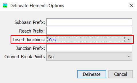
- Make sure the Insert Junctions option is set to "Yes" in the Delineate Elements Options window. This will allow you to retrieve flow data at the outlet of each subbasin.
- For more detailed steps in preprocessing terrain and delineating the watershed, click the link below.
- Make sure the Insert Junctions option is set to "Yes" in the Delineate Elements Options window. This will allow you to retrieve flow data at the outlet of each subbasin.
- Merging and Splitting Elements
- Split and merge subbasins until they are all less than 3 mi2. For more guidance on merging and splitting elements, click the link below.
- Using Merge and Split Tools to Customize Subbasin and Reach Delineation
- Note: The 3 mi2 criteria was used in this model to comply with LA Debris Method EQ 1. However, there are many different debris yield methods that can be used, and each have their own criteria. For other modeling efforts, spend time determining which debris yield method you want to use before continuing with the delineation. The link below talks about 5 methods that are available in HEC-HMS.
- Note: Developing a naming convention for the subbasins, reaches, and junctions helps to easily identify the major drainages within a watershed. This is extremely helpful when correlating stream flow values (peak of a hydrograph) to boundary conditions of a HEC-RAS model.
- Split and merge subbasins until they are all less than 3 mi2. For more guidance on merging and splitting elements, click the link below.
Computing Initial Parameters for the Pre-Fire Model
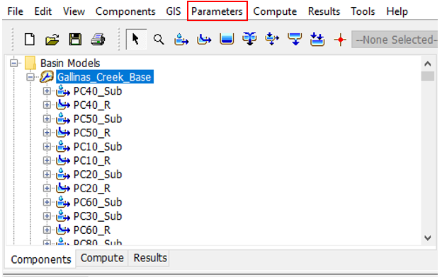
- Now that the watershed has been delineated, it's time to input the initial parameters. To set loss, transform, baseflow, or routing methods, click on your basin model, then click on the Parameters menu.
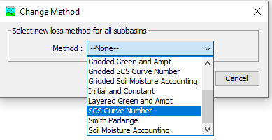
- Select the Parameters | Loss | Change Method menu option. Select Yes to change the method for all subbasins. Select SCS Curve Number method and click the Change button.
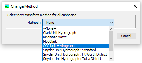
- Select the Parameters | Transform | Change Method menu option. Select Yes to change the method for all subbasins. Select the SCS Unit Hydrograph method and click the Change button.
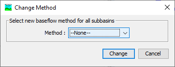
- Select the Parameters | Baseflow | Change Method menu option. Select Yes to change the method for all subbasins. In the Change Method window, select None as the Method. Click the Change button.
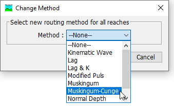
- Select the Parameters | Routing | Change Method menu option. Select Yes to change the method for all reaches. Select the Muskingum-Cunge method and click the Change button.
Loss Method
Select the Soil Conservation Service (SCS) Curve Number (CN) model. The SCS CN model estimates precipitation excess as a function of cumulative precipitation, soil cover, land use, and antecedent moisture. More information about the SCS Curve Number model can be found here: SCS Curve Number Loss Model.
- The Initial Abstraction can be left blank. Leaving the Initial Abstraction blank will result in HEC-HMS automatically calculating the initial loss as 0.2 times the potential retention, which is calculated from the curve number.
- Calculate an area-weighted average Curve Number for each subbasin using the hydrologic soil group (HSG) and land use data. This link demonstrate how to calculate the CN using ArcGIS Pro - Creating a Curve Number Grid and Computing Subbasin Average Curve Number Values.
- Since the CN is a lumped parameter which includes land use, the Percent Impervious is already accounted for and can be left blank or set to zero.
Transform Method
Select the SCS Unit Hydrograph transform model. The SCS Unit Hydrograph model is based on unit hydrographs derived from small watersheds throughout the United States. More information can be found here: SCS Unit Hydrograph Model.
- Leave the Graph Type as "Standard (PRF 484)."
- Note: The peak rate factor (PRF) affects the shape and peak flow of the hydrograph. A higher PRF corresponds to a steep hydrograph with a high peak flow while a lower PRF corresponds to a flatter hydrograph with a lower peak flow.
- The NRCS Hydrology National Engineering Handbook provides equations to calculate the PRF using characteristics of the dimensionless unit hydrograph. In addition, studies have shown that the PRF can vary between 100 and 600, with flat terrain having lower PRFs and mountainous terrain having higher PRFs (NRCS, 2010). If observed flow and precipitation data is available, then different PRFs can be tested when calibrating the model.
- Use equation 15-4a from the NRCS National Engineering Handbook, below, to calculate the initial Lag Time.
- Note: This equation covers a broad span of watersheds, from urbanized to forested. In addition, the watersheds used to develop this equation ranged from 1.3 acres (0.002 mi2) to 9.2 mi2, so the 3 mi2 subbasins used for this model fall within that range (NRCS, 2010).
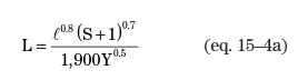
Where L = lag (hrs), l = flow length (ft), Y = average watershed land slope (%), and S = maximum potential retention (in), S=1,000cn'-10, and cn' equals the subbasin area-weighted average Curve Number. - Note: The flow length and average watershed land slope can be taken from the HEC-HMS Subbasin Characteristics as the Longest Flowpath Length (mi) and the Basin Slope (ft/ft) respectively. However, the longest flowpath length must be converted into feet and the basin slope must be converted into percentage.
- Note: This equation covers a broad span of watersheds, from urbanized to forested. In addition, the watersheds used to develop this equation ranged from 1.3 acres (0.002 mi2) to 9.2 mi2, so the 3 mi2 subbasins used for this model fall within that range (NRCS, 2010).
Canopy Method
A canopy method was not utilized because it is accounted for in the CN.
Surface Method
A surface method was not utilized because it is accounted for in the CN.
Baseflow Method
In this study, it was assumed the baseflow was negligible to reduce modeling and calibration time. Since the relative magnitude of the baseflow compared to the magnitude of the flood events is small in the Gallinas Creek Watershed, omitting baseflow would not greatly affect the magnitude of the modeled flood events.
Note: If time permits and the watercourse is perennial, including a baseflow method can improve the accuracy of the model.
Routing Method
Select the Muskingum – Cunge model. The Muskingum – Cunge model was used for the routing because it uses physically-based parameters that can be estimated from stream characteristics.
- Leave the Initial Type as "Discharge = Inflow," which assumes a steady-state initial condition.
- Fill out the Length (ft) and Slope (ft/ft) using the reach characteristics generated in HEC-HMS.
- Locate the reach characteristics by going to Parameters | Characteristics | Reach.
- Note: The Length from the reach characteristics needs to be converted from miles to feet by multiplying by 5,280 feet/mile.
- Set a representative Manning's n value for each reach by looking at aerial imagery and the NLCD - Manning's n values reference table in the HEC-RAS Mapper user manual (link below).
- Leave the Space-Time Method as "auto DX auto DT" so the program automatically selects the appropriate space and time intervals to maintain numeric stability.
- Set the Index Method to "celerity" and set the index celerity to 5 ft/s.
- Note: 5 ft/s is an initial estimate. When running a model simulation, HEC-HMS will report the range of celerity for each reach. You can adjust the celerity if 5 ft/s is outside of the computed range. Otherwise, experiment with celerity to verify results are not sensitive to reasonable celerity values.
- Set the Shape of the reaches to "trapezoid" and estimate the Width and Side Slope by sampling a number of the reach cross sections.
- This tutorial used the Stack Profile tool in ArcGIS Pro to estimate the widths and side slopes of the reaches.
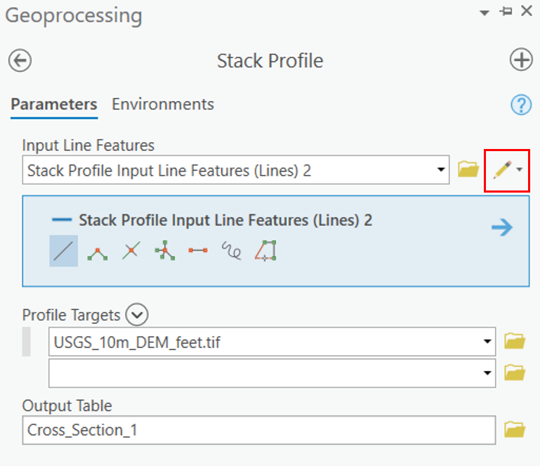
- Select the pencil icon for Input Line Features and draw a cross section line through a reach.
- Set the Profile Targets to the DEM for your study area's terrain, then click Run.
- Next, open the table that was generated and plot the table's "FIRST_DIST" (distance to the first point in the cross section) and "FIRST_Z" (elevation of the point) fields and estimate the width and side slopes of the resulting cross section.
- For more information about the stack profile tool, see the link below:
- This tutorial used the Stack Profile tool in ArcGIS Pro to estimate the widths and side slopes of the reaches.
Meteorological Model
The HEC-HMS meteorologic model can be used to set up boundary conditions for historical storms and for hypothetical floods. Frequency based storms can be created in an HEC-HMS model using the Frequency Storm or Hypothetical Storm precipitation methods. The Hypothetical Storm precipitation method provides the ability to assign different storm durations and temporal patterns.
Hypothetical Storm
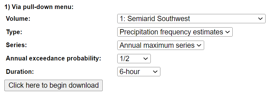
- Download annual maximum precipitation-frequency data for 6 frequencies (annual exceedance probabilities 1% (1/100), 2% (1/50), 4% (1/25), 10% (1/10), 20% (1/5), and 50% (1/2)) from the NOAA Atlas 14 website (PF in GIS Format - PFDS/HDSC/OWP).
- Set the volume to the region of the study area (Semiarid Southwest for this tutorial).
- Set the duration to 6 hours.
- For more guidance on downloading and importing NOAA Atlas 14 precipitation-frequency gridded data, see the tutorial below.
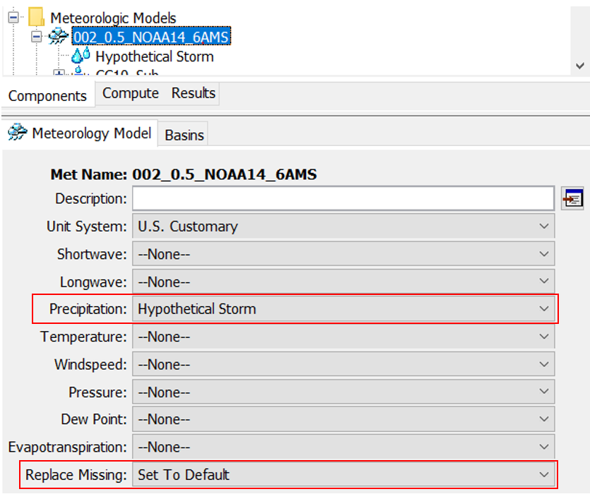
- Create a Meteorologic Model by navigating to Components | Meteorologic Model Manager. Click New in the Meteorologic Model Manager window and name the meteorologic model something to indicate the frequency. In this tutorial "002_0.5_NOAA14_6AMS" is used for a precipitation event with an annual exceedance probability of 50%.
- Click on the newly created meteorological model, which can be found in the Meteorological Models folder in the Components tab.
- Set the Precipitation to "Hypothetical Storm" and Replace Missing to "Set To Default."
- Set the Precipitation to "Hypothetical Storm" and Replace Missing to "Set To Default."
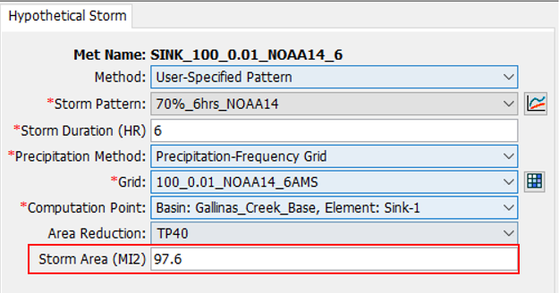
- Enter the parameters for the hypothetical storm by clicking on Hypothetical Storm.
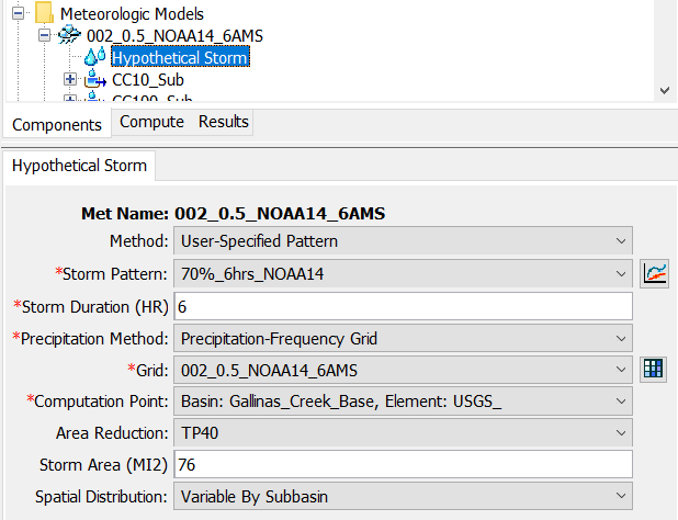
- Set the Method to "User-Specified Pattern." This allows you to input your own storm time pattern.
- Input a Storm Pattern. The storm pattern describes how total storm depth is distributed incrementally throughout the storm event. Two methods of developing a temporal pattern are described below.
- NOAA Atlas 14 temporal patterns: NOAA Atlas 14 contains temporal patterns developed by processing regional storm events.
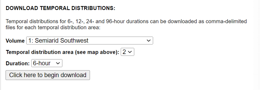
- Download the temporal distribution spreadsheet for the desired volume, area, and duration from NOAA Atlas 14 website linked below.
- Note: Make sure to select the correct volume and temporal distribution area for your study area. This tutorial uses volume 1, and temporal distribution area 2.
- Using the downloaded spreadsheet, choose a temporal distribution that represents observed events in the region.
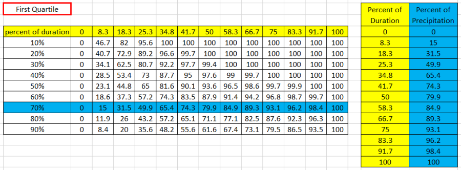
- For the Gallinas Watershed model the 1st quartile temporal pattern was used because most of the observed storms were front-loaded.
- The first column (with values of 10% to 90%) indicates the cumulative probability of occurrence for each temporal distribution. For this tutorial, sensitivities for multiple temporal distributions were run, and the 1st quartile 70% temporal distribution was ultimately selected. Before entering the temporal pattern into HEC-HMS, you will need to create a paired data table with "percent of storm duration" vs "percent of total storm depth" as shown below.
- Historical storms can be used to create normalized temporal patterns. See the tutorial below for details on developing a storm pattern based on a historical event.
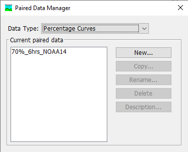
- Create the NOAA Atlas 14 distribution pattern by navigating to Components | Paired Data menu and selecting the Percentage Curves data type. Click New... in the Paired Data Manager window and name the paired data "70%_6hrs_NOAA14".
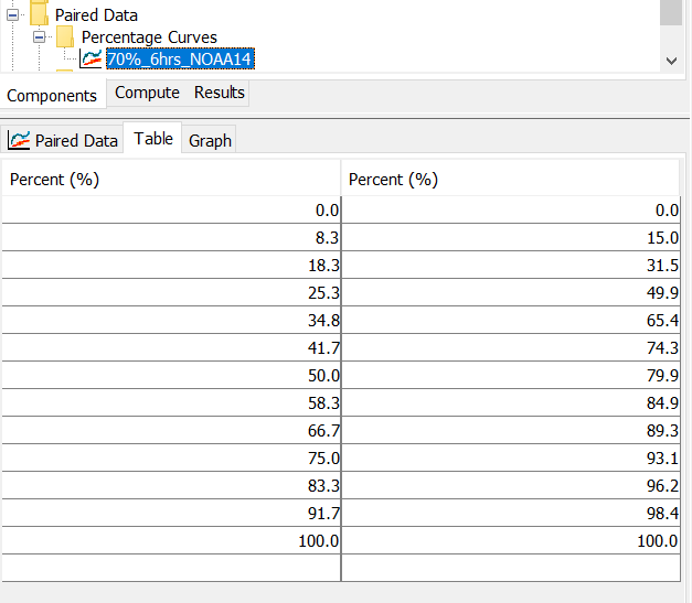
- Navigate to the newly created percentage curve by clicking on the folders called Paired Data | Percentage Curves.
- Add the percent of duration (first column) and percent of total precipitation (second column) of the selected quartile and percentage (in this case the 1st quartile 70%) to the Table tab.
- NOAA Atlas 14 temporal patterns: NOAA Atlas 14 contains temporal patterns developed by processing regional storm events.
- Set the Storm Duration to 6 hours.
- Note: Rule of thumb is to make sure the duration is 2-3 times longer than the time of concentration at the computation point.
- Set the Precipitation Method to "Precipitation-Frequency Grid" because the NOAA Atlas 14 precipitation-frequency gridded data is being used for this tutorial.
- Set the Grid to the gridded data with the correct frequency.
- Set the Computation Point. In this tutorial, the computation point is the USGS gage because we are interested in the peak discharges at this point.
- Apply an Area Reduction. For this tutorial, TP40 was used.
- Add a Storm Area.
- The storm area is the drainage area of the computation point.
- Note: The model results will only be accurate at the computation point with the inputted area reduction. If the values of another point in the watershed are needed, a new meteorological model needs to be created with the appropriate computation point and area reduction. This is a consideration when defining junction locations in the model, so an area reduction can be applied to all locations where streamflow will be extracted.
- Set the Spatial Distribution as "Variable by Subbasins."
- Create five more meteorological models for the remaining frequencies and name them accordingly.
- For more guidance on creating a hypothetical storm, see the tutorial below.
Frequency storm
- The frequency storm can be used as an alternative to the hypothetical storm meteorological model. You will need to use the frequency storm option when using debris flow methods that are sensitive to short duration precipitation. The frequency storm option allows you to directly define precipitation depths over a range of storm durations.
- The tutorial below includes steps on how to import precipitation frequency grids and how to populate the frequency storm meteorological model.
Creating a Frequency Analysis for Pre-Fire Conditions
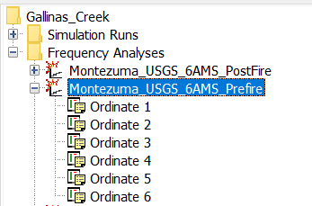
- Create a frequency analysis for pre-fire conditions by selecting Compute | Create Compute | Frequency Analysis.
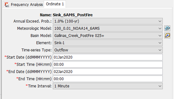
- Create an ordinate for each frequency by right clicking on the frequency analysis and selecting Add Ordinate.
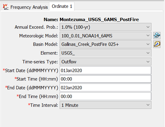
- Fill out the information for each frequency (see below for the 1% annual exceedance probability event).
- The Element is the location where the discharge will be computed (In this model, the location of a USGS gage will be used to calibrate the model). The appropriate element must be selected in order for the correct area reduction factor to be computed.
- The Start Date and Start Time do not matter, but an End Date and End Time should be chosen so the frequency analysis can capture the entire hydrograph for every subbasin within the watershed.
- For this tutorial, 24 hours is sufficient.
- Selecting the appropriate Time Interval for the simulation is important for capturing the peak of the hydrograph. If your watershed is steep or has quickly rising hydrographs, a smaller time interval is needed.
- A time interval of 1 minute was used for this tutorial.
- A time interval of 1 minute was used for this tutorial.
- Create an ordinate for each frequency by right clicking on the frequency analysis and selecting Add Ordinate.
Calibrating the Pre-Fire Model
Calibrating to a Discharge-Frequency Curve
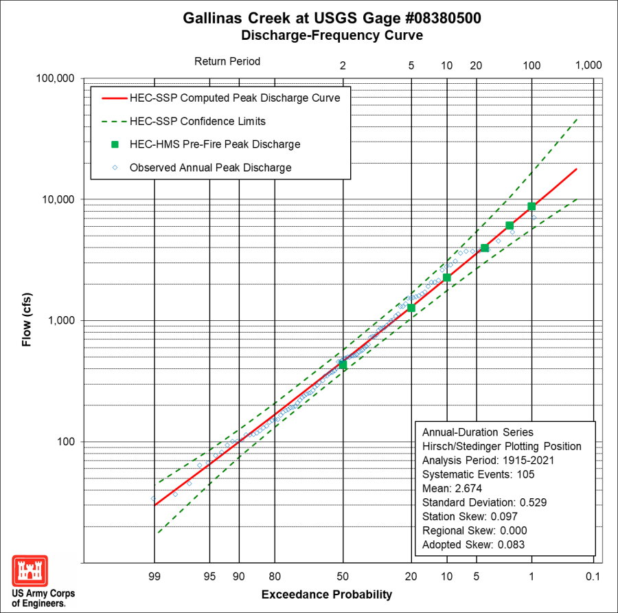
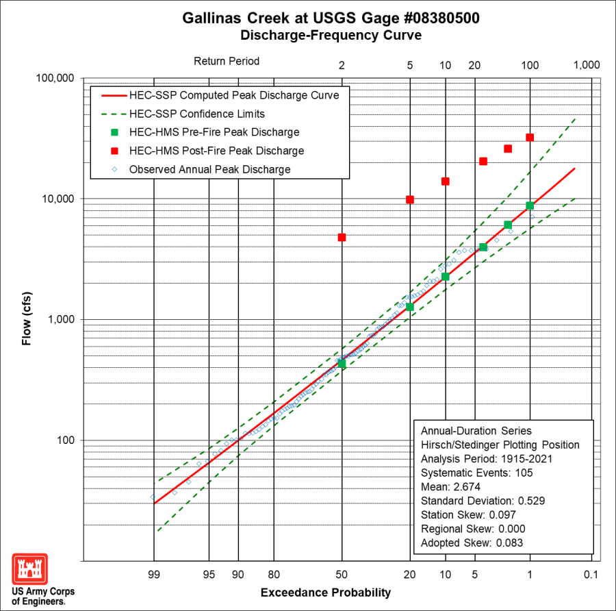
Calibrate the peak flows computed in HEC-HMS to the discharge-frequency curve developed in Discharge-Frequency Curve Development Using HEC-SSP.
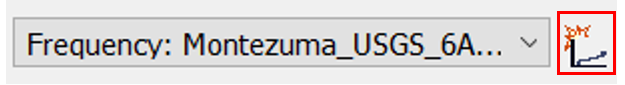
- Run the frequency analysis by clicking on the compute icon (shown below).
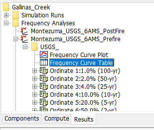
- After computing the frequency analysis, view the results by clicking on the Frequency Curve Table in the Results tab.
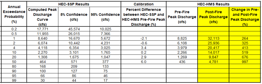
- Use the "Discharge Frequency Curve" spreadsheet to visualize the difference between the HEC-HMS peak discharges and the HEC-SSP discharge-frequency curve. The spreadsheet contains the computed curve and the confidence limits that were developed in HEC-SSP using annual peak discharge data from a USGS gage within the Gallinas Creek Watershed.
- Add the results from the Frequency Curve Table to the "Pre-Fire Peak Discharge" column to see how the values compare to the HEC-SSP results.
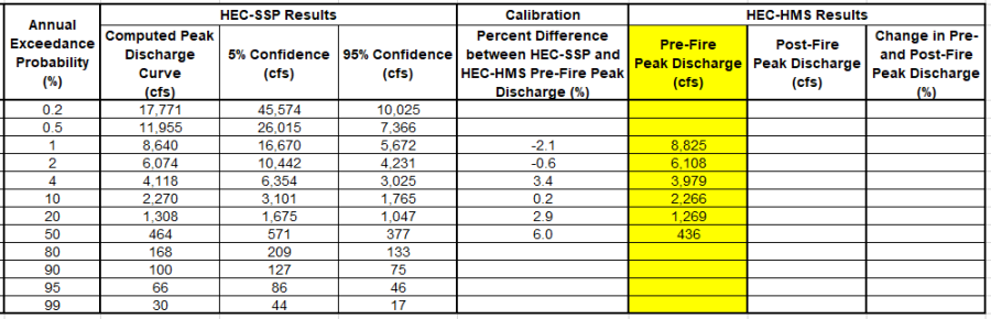
- Add the results from the Frequency Curve Table to the "Pre-Fire Peak Discharge" column to see how the values compare to the HEC-SSP results.
- Make small adjustments to the CN values by multiplying each subbasin's CN value by a constant adjustment factor and recompute the lag using the new CN values (see "Transform Method" section for lag equation). Repeat this process until the magnitude and trends of the peak flows computed in the HEC-HMS model are reasonably close to the discharge-frequency curve.
- If the discharge values computed in HEC-HMS are too high, decrease the curve numbers. If they're too low, increase the curve numbers.
- Separate basin models with unique CN values and lag times can be created for different event frequencies to achieve a better calibration.
- In this tutorial, the computed lag was reduced by 10% for events with an annual exceedance probability of 1% - 4% to account for the expected decrease in lag time with an increase in event magnitude.
- Once the CN values and lag times are adjusted and the model calibrated to the discharge-frequency curve, these peak flow values serve as the calibrated pre-fire conditions for the watershed. Adjustments made to reflect the post-fire conditions of the watershed will be applied to these calibrated pre-fire values.
- Some watersheds do not have gages with observed flow for calibration; however, below are some alternative ways to develop a discharge-frequency curve.
- Regional regression equations can be used to develop a discharge-frequency curve.
- StreamStats (link below) is a USGS tool that can be used to delineate many watersheds in the United States and generate their peak flow statistics using regional regression equations. StreamStats can also calculate various other basin characteristics, such as drainage area and mean annual precipitation.
- A gage from a nearby watershed can be used by scaling the gage's flow by a ratio of the drainage area of the gage to the drainage area of the watershed you are modeling.
- Make sure the characteristics of the gage's drainage area are similar to the characteristics of the watershed you are modeling.
- The size of the gage's and watershed's drainage areas should be similar. It is not recommended to use a gage if its drainage area is less than 50% or over 150% of your modeled watershed's drainage area.
- Regional regression equations can be used to develop a discharge-frequency curve.
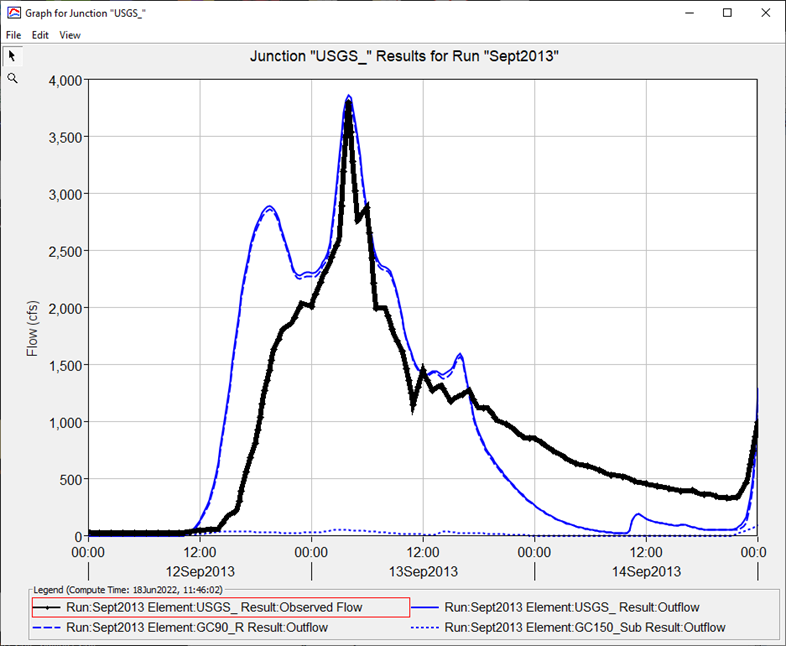
Calibrating to an Observed Event
If time allows, the model can be calibrated to observed events by using observed precipitation and stream gage data. (Note: This calibration method was not used to determine the final calibrated parameters in the Gallinas Creek model and is only included to provide an example of an alternative calibration method for future modeling efforts).
- Add observed discharge data to the model.
- Download the GallinasC.dss file, which contains 15-minute discharge data from 1990 to 2021.
- Create a new time-series for the discharge gage and set the data source to the dss file. For more details on setting up the discharge gage time-series, click the link below.
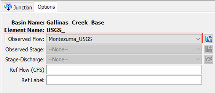
- Add the observed flow to the element representing the gage in the model.
- Click on the element in the basin model, then go to the Options tab.
- Set the Observed Flow to the newly created discharge gage time-series.
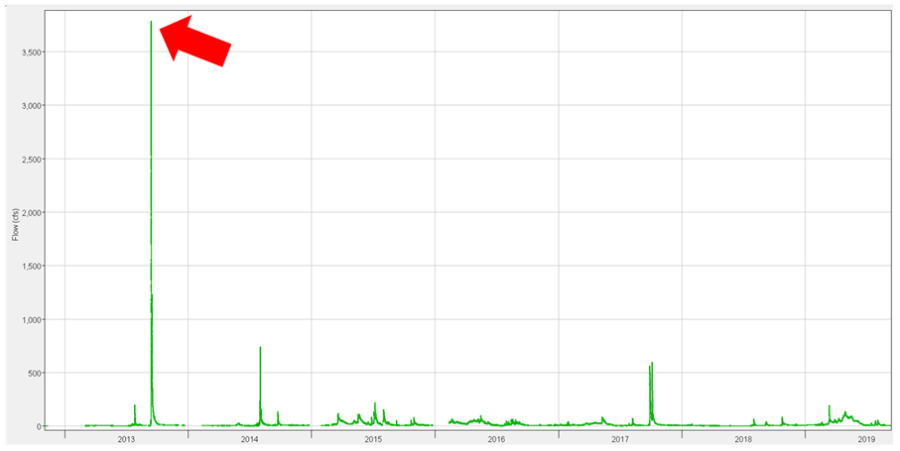
- Determine which observed event to use in the calibration.
- Look at the discharge data and choose an event with a large peak discharge.
- For this model, the September 12-15, 2013 event will be used.
- Create a "Gridded Precipitation" meteorological model.
- Add gridded precipitation to the model.
- Download gridded precipitation data for September 2013 from the NOAA website (Link below).
- Index of /aorc-historic/AORC_WGRFC_4km/WGRFC_precip_partition (noaa.gov)
- Other gridded precipitation sources are described in the link below.
- Import the gridded precipitation data and add it to the meteorological model.
- Note: Make sure you know the time zone of the gridded precipitation. The AORC precipitation used for the Gallinas Creek model is in the coordinated universal time (UTC), which is 6 hours ahead of MDT (the time zone of the September 2013 event). The time shift can be easily applied by expanding the meteorological model, clicking on Gridded Precipitation, and entering the time shift in hours.
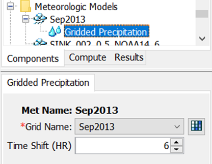
- Note: Make sure you know the time zone of the gridded precipitation. The AORC precipitation used for the Gallinas Creek model is in the coordinated universal time (UTC), which is 6 hours ahead of MDT (the time zone of the September 2013 event). The time shift can be easily applied by expanding the meteorological model, clicking on Gridded Precipitation, and entering the time shift in hours.
- Download gridded precipitation data for September 2013 from the NOAA website (Link below).
- Add gridded precipitation to the model.
- Set up a control specification for the September 2013 event.
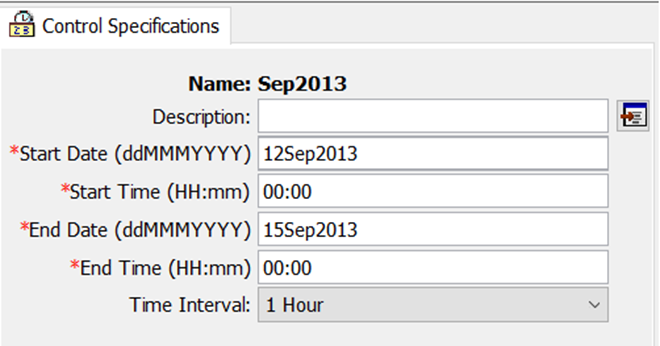
- Create a simulation run with the basin model, control specifications, and meteorological model for the September 2013 event.
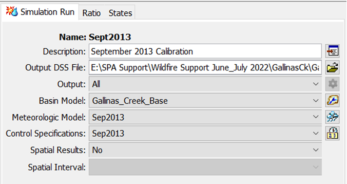
- Adjust the loss, transform, and baseflow parameters until the computed flow matches the magnitude, timing, and shape of the observed flow hydrograph.
- Note: For calibration to known events, inclusion of a baseflow may be useful to facilitate convergence of the modeled to observed results.
- Note: For calibration to known events, inclusion of a baseflow may be useful to facilitate convergence of the modeled to observed results.
- For more detailed steps on importing gridded data, creating a meteorological model, and setting up a simulation run, click the link below.
- Importing and Using Daymet Precipitation Data
- The tutorial linked above uses Daymet data, but the methodology can be applied to any type of gridded data.
- Importing and Using Daymet Precipitation Data
Post-Fire Model Setup
- Create post-fire basin models by adjusting the CN values and lag times to reflect post-fire conditions.
- For the Gallinas Creek model, the pre-fire CN values were converted to post-fire CN values using burned area emergency response (BAER) soil burn severity maps and relationships developed by Livingston et al. (2005). This approach requires the following steps:
- Determine the percentage of area that has a low, moderate, and high burn severity for each subbasin.
- Click the link below for detailed steps on calculating burn severity percentages.
- A relationship was developed by Livingston et al. using fires in New Mexico that defines a wildfire hydrologic impact (WHI) factor based on the percentage of subbasin area that has a high burn severity versus a moderate burn severity.
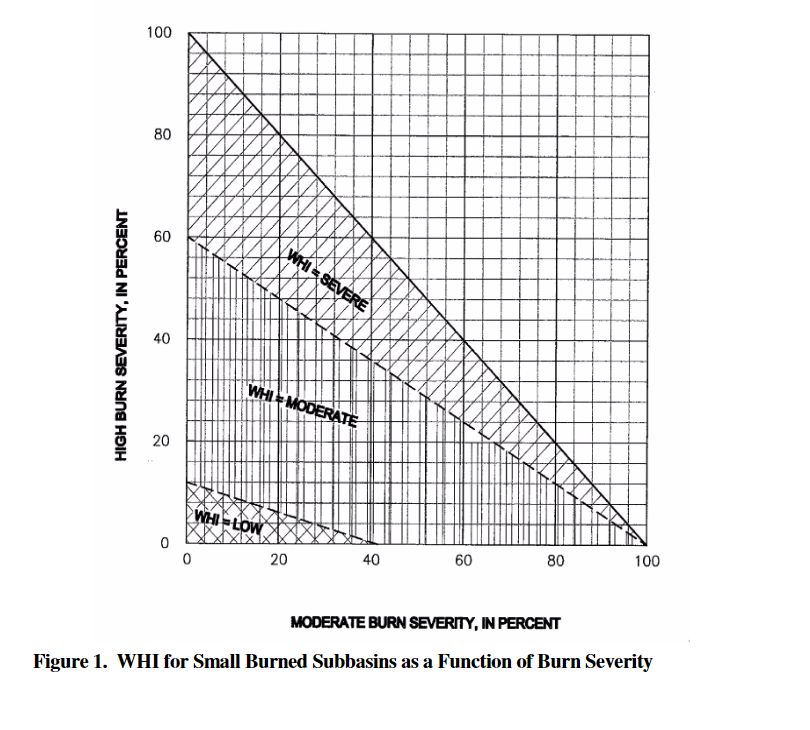
- Determine the percentage of area that has a low, moderate, and high burn severity for each subbasin.
- A second relationship was developed by Livingston et al. using data from New Mexico and Southwestern Colorado fires to relate pre- and post-fire CNs for each WHI factor (Livingston et al., 2005). This relationship was used to determine the appropriate initial CN ratio to apply to each subbasin to compute the post-fire CN.
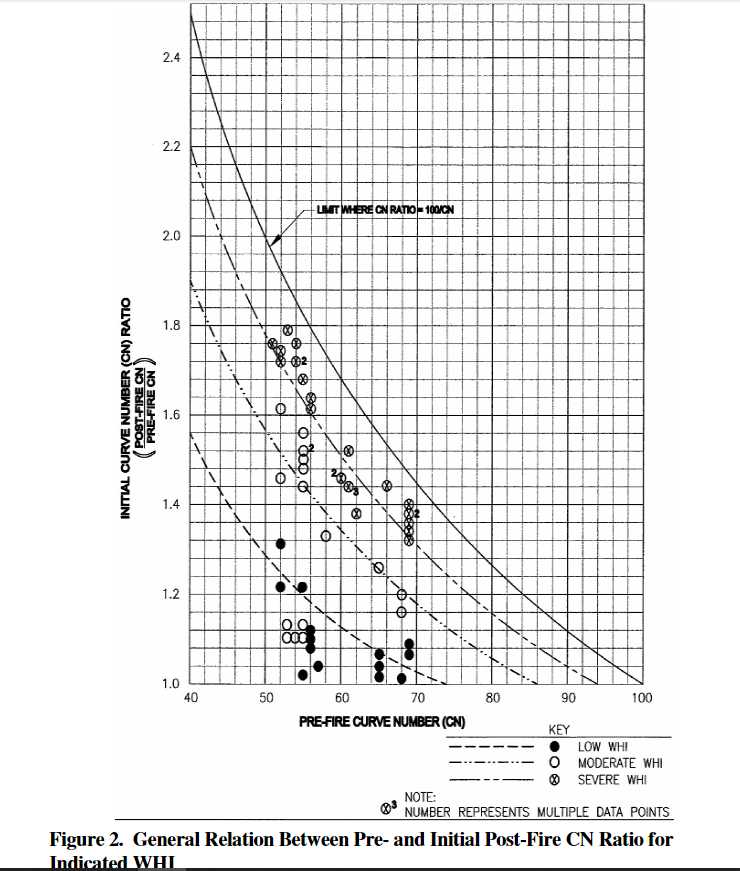
- Computing the initial CN ratio for every subbasin by hand is unrealistic, so a spreadsheet was developed to automate the process.
- Download the "Post-Fire_CN_Values_GCW" spreadsheet.
- Enter the subbasin names, pre-fire CN values, and % of high, moderate, low, and unburned area in the "Inputs" tab.
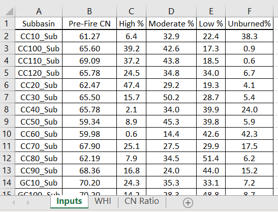
- The rest of the spreadsheet will automatically populate, and the resulting post-fire CN values will be highlighted in the "CN Ratio" tab.

- Create post-fire basin models for each frequency.
- Copy the pre-fire basin models by right clicking on the pre-fire basin models and selecting Create Copy...
- Change the CN values to the post-fire values and recompute the lag using the post-fire CN values.
- In this tutorial, the computed lag was reduced by 10% for events with an annual exceedance probability of 1% - 4% to account for the expected decrease in lag time with an increase in event magnitude.
- Create a frequency analysis for post-fire conditions.
- See the "Frequency Analysis" section for detailed steps.
- Use the "Discharge Frequency Curve" spreadsheet to visualize the difference between pre- and post- fire discharges.
Calculating Water Volume at the Watershed Outlet
- It is often desirable to provide inundation extents for the modeled rainfall-runoff events. Since the transport of debris after the wildfire can be large, it is recommended to bulk the flow or otherwise account for the increased volume of moving fluid within the hydraulic model being used to determine the inundation extents. The estimation of a bulking factor may be done anywhere within the developed hydrologic model and should correlate to a location consistent with the input flow values for the hydraulic modeling. For the Gallinas Creek model the outlet location was chosen to provide a bulking factor for the entire watershed. Note that the chosen locations may need a new frequency analysis that has the appropriate area reduction factor applied.
- Since the USGS gage used to calibrate the Gallinas Creek model is not at the outlet of the watershed, another frequency analysis needs to be conducted. The water volume at the outlet location is needed to compute the bulking factor.
- Create a new set of hypothetical storm meteorological models and set the Storm Area to the total drainage area of the Gallinas Creek Watershed. In some cases you do not need to follow this step. The Frequency Analysis allows you to choose an Element for each Ordinate. The drainage area of the Element overwrites the Storm Area defined in the Hypothetical Storm component editor.
- Create a new frequency analysis using the post-fire basin models and the meteorological models.
- Run the frequency analysis and view the results in the Results tab.
References
Livingston, R., Earles, T., and Wright, K., 2005. Los Alamos Post-Fire Watershed Recovery: A Curve-Number-Based Evaluation. Watershed Management Conference 2005, ASCE Library. https://ascelibrary.org/doi/10.1061/40763%28178%2941
NOAA, 2017a. NOAA Atlas 14 Precipitation Frequency Estimates in GIS Compatible Format. NOAA's National Weather Service, Hydrometeorological Design Studies Center, Precipitation Frequency Data Server (PFDS). April 21, 2017. https://hdsc.nws.noaa.gov/hdsc/pfds/pfds_gis.html
NOAA, 2017b. Temporal Distributions for 6-, 12-, 24- and 96-hour Durations. NOAA's National Weather Service, Hydrometeorological Design Studies Center, Precipitation Frequency Data Server (PFDS). April 21, 2017. https://hdsc.nws.noaa.gov/hdsc/pfds/pfds_temporal.html
NRCS, 2010. Part 630 Hydrology National Engineering Handbook: Chapter 15 Time of Concentration. Natural Resources Conservation Service, United States Department of Agriculture. Washington D.C.
Project Files
Download the final project files here:
Discharge_Frequency_Curve_GCW_final.xlsx
